In the grammar of graphics, the term “scale” refers to the specific rule that converts data values into visual properties. This chapter explores the various types of scales applicable for different data and aesthetic mappings:
Many statistical variables are continuous, representing measurements that can vary smoothly across a range, such as distance, time, and temperature. These variables are often denoted with a decimal point to reflect their observed value. However, for practical purposes, continuous variables are sometimes rounded to a discrete set of values. For instance, a person’s age, while technically continuous, is commonly reported in whole years for simplicity.
Conversely, some variables are inherently discrete, meaning they can assume only specific, separate values. For example, the number of seats on a passenger plane must be an integer. However, in the context of ggplot2, all numeric columns in a data frame, whether continuous or discrete, are treated as continuous variables. In contrast, ggplot2 classifies columns of logical and character vectors, as well as factors, as discrete variables.
This section takes a detailed look at scales tailored for continuous variables, such as x-coordinates, y-coordinates, and legends for color and size. Section 9.1.1 will guide you through adjusting the limits of continuous scales. Section 9.1.2 will focus on customizing the breaks and labels. The scales package offers a suite of helper functions for labels, introduced in Section 9.1.3. A particularly crucial scale is the logarithmic transformation, which is the focus of Section 9.1.4.
9.1.1 Setting Scale Limits
To create an example with several continuous scales, consider the following subset, named demographics, of the gapminder data set, focusing on life expectancy and GDP per capita in three Southeast Asian countries—Indonesia, Malaysia, and Singapore:
# A tibble: 36 × 6
   country   continent  year lifeExp       pop gdpPercap
   <fct>     <fct>     <int>   <dbl>     <int>     <dbl>
 1 Indonesia Asia       1952    37.5  82052000      750.
 2 Indonesia Asia       1957    39.9  90124000      859.
 3 Indonesia Asia       1962    42.5  99028000      849.
 4 Indonesia Asia       1967    46.0 109343000      762.
 5 Indonesia Asia       1972    49.2 121282000     1111.
 6 Indonesia Asia       1977    52.7 136725000     1383.
 7 Indonesia Asia       1982    56.2 153343000     1517.
 8 Indonesia Asia       1987    60.1 169276000     1748.
 9 Indonesia Asia       1992    62.7 184816000     2383.
10 Indonesia Asia       1997    66.0 199278000     3119.
# ℹ 26 more rows
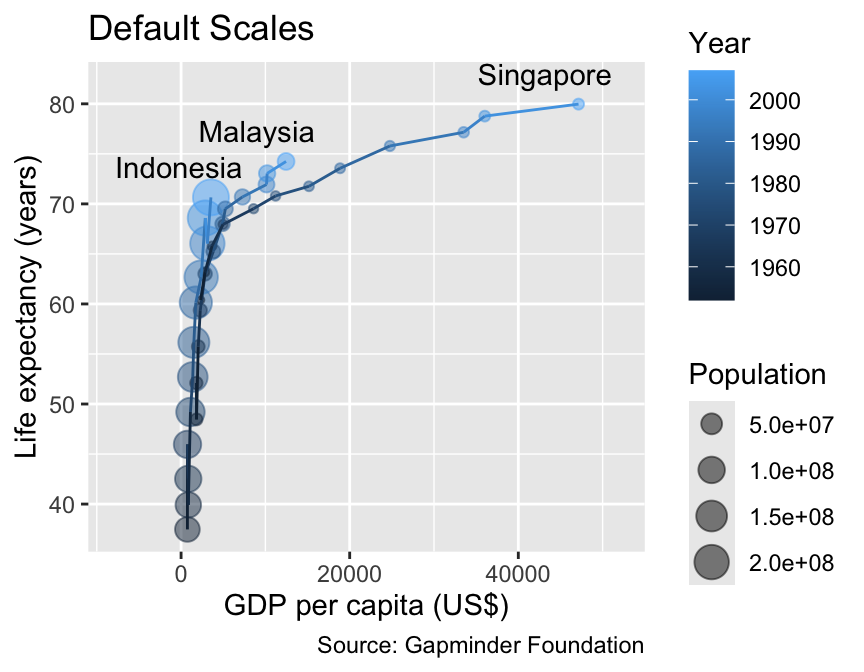
The following plot visualizes four quantitative variables:
GDP per capita as x-coordinate
Life expectancy as y-coordinate
Year as color
Population as size
It is noteworthy that year and pop, represented by integers, are mathematically discrete but will be interpreted as continuous by ggplot2.
All numerical variables, including integers, are treated as continuous by ggplot2.
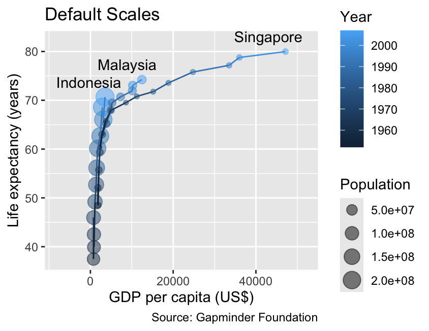
The code below uses the group aesthetic, introduced in Section 8.7, to generate a separate line for each country:
gg_demographics<-ggplot(demographics,aes(x =gdpPercap, y =lifeExp, color =year, group =country))+geom_point(aes(size =pop), alpha =0.5)+geom_line()+geom_text(aes(label =country), data =slice_max(demographics, year), color ="black", hjust =0.75, # Horizontal justification toward the left vjust =0, # Vertical justification toward the top nudge_y =2)+labs( x ="GDP per capita (US$)", y ="Life expectancy (years)", color ="Year", size ="Population", title ="Default Scales", caption ="Source: Gapminder Foundation")+xlim(-8000, 52000)gg_demographics
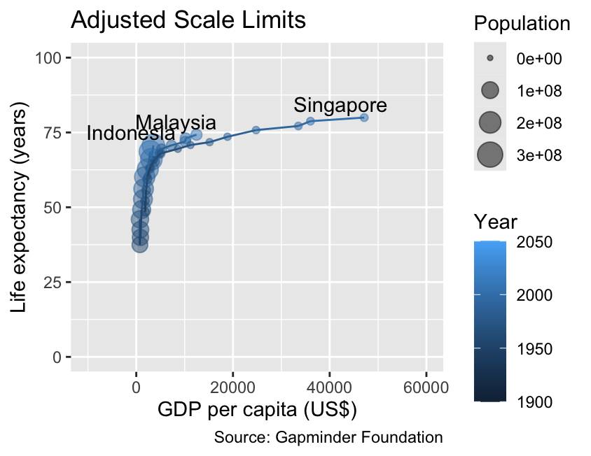
The scales associated with continuous variables can be customized using the scale_*_continuous() functions, where * is replaced with the name of the aesthetic. For example, the code below illustrates how to adjust the limits for both spatial coordinates, as well as the scales for color and size. For the moment, please disregard the fact that ggplot2 reverses the order of the size and color legends. Instructions on how to reorder legends will be provided in Section 10.2:
Use the scale_*_continuous() functions to customize continuous scales.
The limits argument of the scale_*_continuous() functions adjusts the plotted range of values.
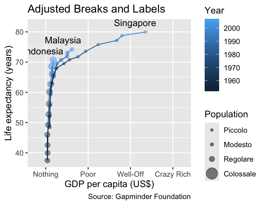
9.1.2 Setting Scale Breaks and Labels
Adjusting breaks and labels is a key aspect of customizing the scale_*_continuous() functions beyond setting limits. For x-coordinates, y-coordinates, and color bars, breaks are indicated by tick marks—short lines that extend perpendicularly from the axis or legend. In contrast, for scales representing size or line width, breaks are visually differentiated by symbols of varying sizes. In this context, a “label” refers to a text annotation next to a break (e.g., “20000” on the x-axis in the plot below). Additionally, the x-axis and y-axis may feature minor breaks, depicted as thin grid lines without accompanying tick labels.
Use the breaks, minor_breaks, and labels arguments of the scale_*_continuous() functions to customize breaks and labels of continuous scales.
gg_demographicsgg_demographics+labs(title ="Adjusted Breaks and Labels")+scale_x_continuous( breaks =seq(from =0, to =60000, by =20000), minor_breaks =NULL, # Remove minor breaks labels =c("Nothing", "Poor", "Well-Off", "Crazy Rich"), limits =c(-5000, 65000))+scale_size_continuous( breaks =10^(6:9), labels =c("Piccolo", "Modesto", "Regolare", "Colossale"), limits =c(0, 1e9))
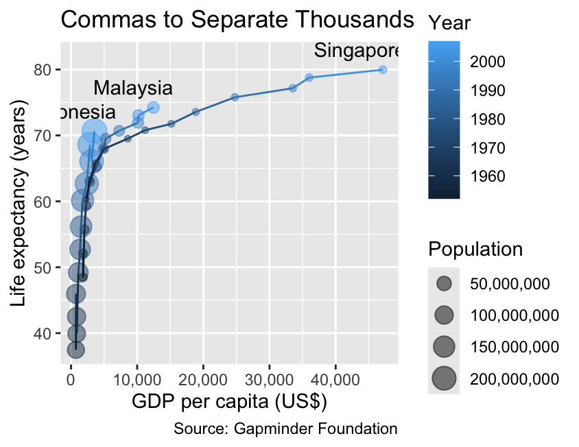
9.1.3 Functions for Labels in the scales Package
The scales package offers a collection of utility functions for commonly required label modifications. For example, label_comma() improves the readability of large numbers by inserting commas to demarcate blocks of three digits and ensures that numbers are displayed in full decimal notation rather than scientific notation like “1.0e+08”. Please note that label_comma() reduces the padding of the x-coordinates in the plot below, partly obscuring the labels “Indonesia” and “Singapore.” In production code, you might need to adjust the padding manually using the expand argument of the scale_x_continuous() function:
Use the scales package’s helper functions to refine and customize labels.
library(scales)gg_demographicsgg_demographics+labs(title ="Commas to Separate Thousands")+scale_x_continuous(labels =label_comma())+scale_size_continuous(labels =label_comma())
Use label_comma() to insert commas to separate blocks of three digits.
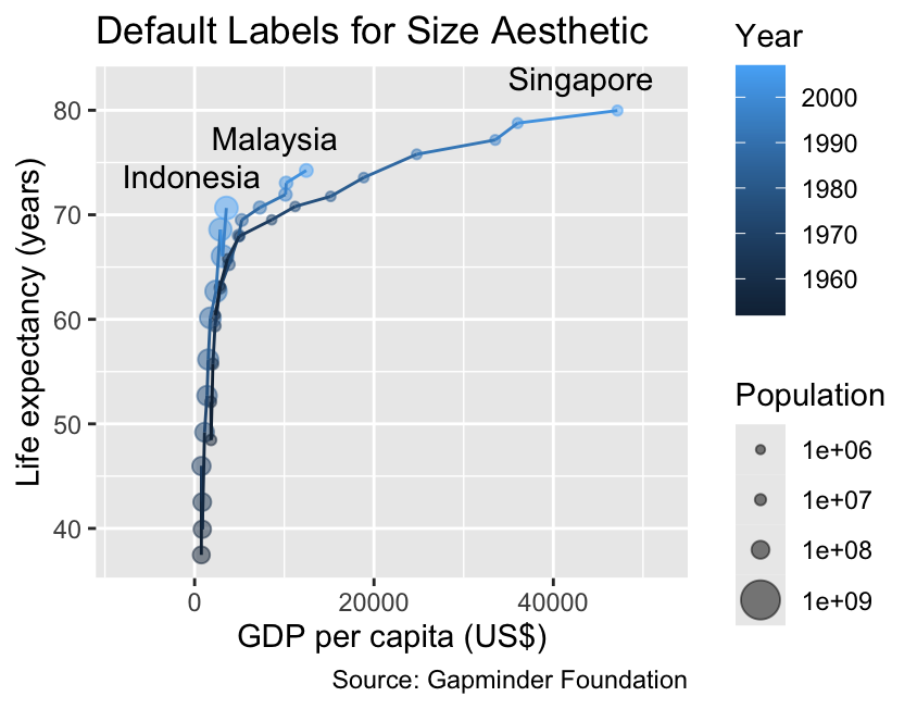
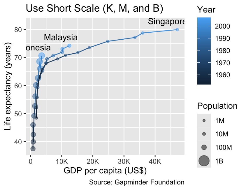
The label_number() function, when used with the scale_cut = cut_short_scale() argument, provides an alternative that can often enhance label legibility even further. It abbreviates “thousand” as “K,” “million” as “M,” “billion” as “B,” and “trillion” as “T,” emphasizing the scale of the values being represented:
Use label_number(scale_cut = cut_short_scale()) to abbreviate large numbers (e.g., “thousand” as “K”).
gg_demographics+labs(title ="Default Labels for Size Aesthetic")+scale_size_continuous( breaks =10^(6:9), limits =c(0, 1e9))gg_demographics+labs(title ="Use Short Scale (K, M, and B)")+scale_x_continuous(labels =label_number(scale_cut =cut_short_scale()))+scale_size_continuous( breaks =10^(6:9), labels =label_number(scale_cut =cut_short_scale()), limits =c(0, 1e9))
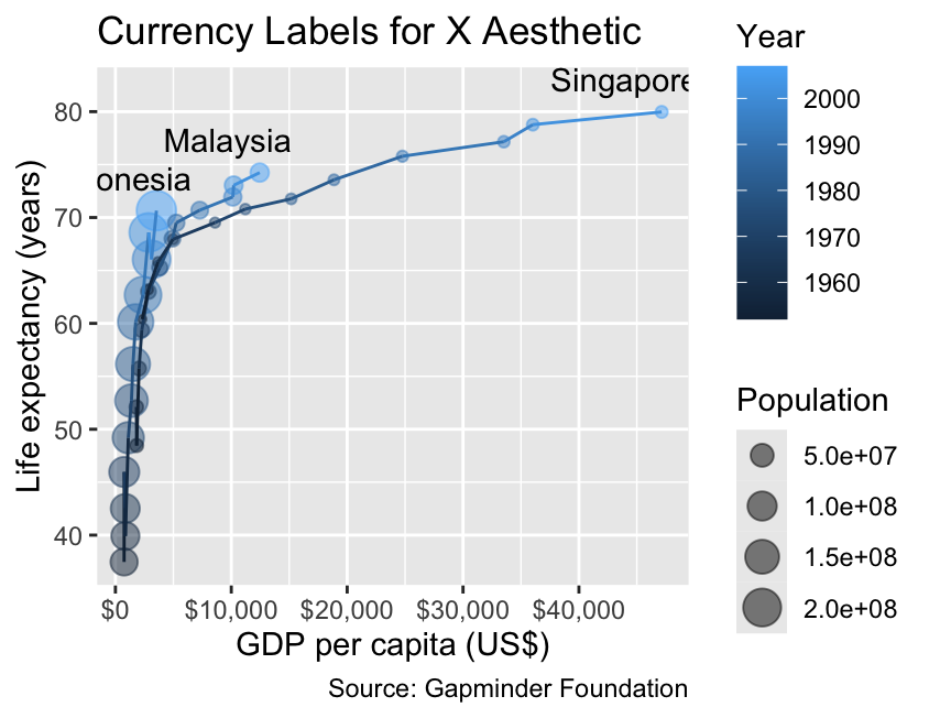
The label_currency() function formats numbers as currency values, adding a dollar sign by default and grouping thousands with commas for readability. While indicating the currency next to the value can often improve readability, one might argue that the dollar signs in front of the numbers are redundant in this example because the axis title already indicates the currency (“US$”):
Use label_currency() to add a currency sign (e.g., “$” or “€”) and separate thousands with commas.
gg_demographicsgg_demographics+labs(title ="Currency Labels for X Aesthetic")+scale_x_continuous(labels =label_currency())
9.1.4 Logarithmic Scales
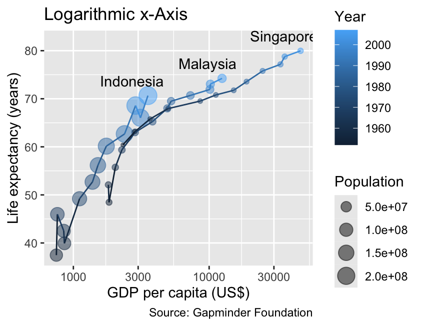
Real-world data often span a wide range of magnitude. For right-skewed distributions, where most values are small but a few are much larger, logarithmic scales can help reveal patterns by transforming data. Logarithmic scales can be generated using the scale_x_log10() and scale_y_log10() functions. The following code applies a logarithmic scale to the x-axis, resulting in a graph that is less curved and has fewer overlapping data points:
For right-skewed data, consider using scale_x_log10() and scale_y_log10() to apply logarithmic transformations to the coordinate axes.
When using logarithmic scales, it is conventional to print large and small numbers in superscript format (e.g., 104 instead of 1e+04). The label_log() function from the scales package can assist you with this task. We will use label_log() to format the y-axis labels in the subsequent code example.
Use label_log() from the scales package to display large and small numbers in superscript formatting (e.g., 104).
Like x-scales and y-scales, color scales can also be log-scaled, as illustrated by the following code. However, as discussed in Section 8.1.2, color can only be meaningfully mapped to intensive data, such as per-capita GDP. The code below uses the breaks_log() argument from the scales package to generate a sequence of nearly equidistant breaks on a logarithmic scale.
Use breaks_log() from the scales package to generate a sequence of nearly equidistant breaks for a logarithmic scale.
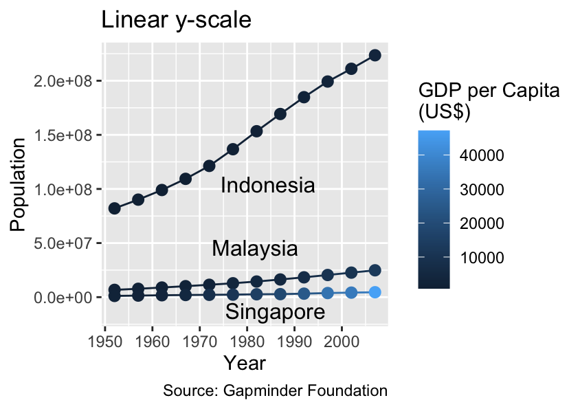
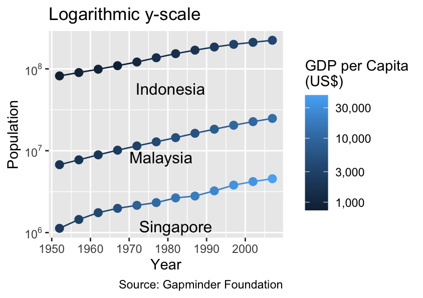
Logarithmic scales are not ideally suited for size or line width because our perception of these visual properties is additive, whereas the log-transformation is nonlinear. For extensive data with a right-skewed distribution, such as country populations, it is preferable to map them to spatial coordinates rather than size aesthetics to prevent misinterpretation. The following plot implements this idea:
gg_time_series<-ggplot(demographics,aes( x =year, y =pop, color =gdpPercap, label =country, group =country))+geom_line()+geom_point(size =2.5)+# Increase point sizedirectlabels::geom_dl(method ="smart.grid", color ="black")+labs( x ="Year", y ="Population", color ="GDP per Capita\n(US$)", # Line break ("\n") in label caption ="Source: Gapminder Foundation")gg_time_series+labs(title ="Linear y-scale")+ylim(-1.5e7, NA)gg_time_series+labs(title ="Logarithmic y-scale")+scale_y_log10(labels =label_log())+scale_color_continuous( breaks =breaks_log(), labels =label_comma(), transform ="log10")
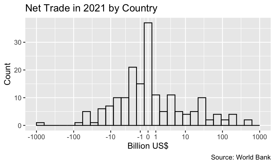
Note that the logarithm is only defined for positive values. If your data contain non-positive values, you might want to consider using a “symmetric logarithmic” transformation instead. The following example illustrates how to apply this transformation using the scales package’s pseudo_log_trans() function. The example depicts the distribution of net trade by country in 2021, which ranges from approximately -1 trillion to 1 trillion US dollars. You can download the data in XLS format from the textbook website:
net_trade<-"net_trade.xls"|>readxl::read_xls(skip =3)|>select(usd =`2021`)|>mutate(billion_usd =usd/1e9)|>drop_na()ggplot(net_trade, aes(billion_usd))+geom_histogram(bins =30, fill =NA, color ="black")+labs( x ="Billion US$", y ="Count", title ="Net Trade in 2021 by Country", caption ="Source: World Bank")+scale_x_continuous( breaks =c(-10^(3:0), 0, 10^(0:3)), limits =c(-1e3, 1e3), transform =pseudo_log_trans(base =10),)
9.1.5 Section Summary: Continuous Scales
This section showed how to tailor scales using the scale_*_continuous() functions. It illustrated the use of various arguments such as breaks, minor_breaks, labels, and limits to refine the presentation of axes and legends. The scales package offers various helper functions for common modifications of breaks and labels. Additionally, the chapter discussed the use of logarithmic scales for axes and color bars, which is particularly beneficial for right-skewed data spanning a wide range of magnitudes.
9.2 Discrete Scales
Discrete scales in ggplot2, which apply to variables in the logical, character, and factor classes, can be customized using the scale_*_discrete() functions. Like the scale_*_continuous() functions, they possess arguments for limits (Section 9.2.1), breaks (Section 9.2.2), and labels (Section 9.2.3), which allow for fine-tuning of the scales’ appearance and behavior.
Use the scale_*_discrete() functions to customize discrete scales in ggplot2.
9.2.1 Limits
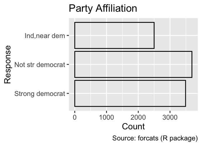
The limits argument defines the possible values for a discrete scale. Unlike for continuous scales, where the limits argument requires the specification of the scale’s endpoints only, discrete scales require a limits argument with as many elements as there are categories in the plot. If the data includes values not specified in limits, ggplot2 will issue a warning. For example, the following code shows the party affiliation of GSS participants; when the y-axis is limited to three categories, a warning is printed:
Use the limits argument to specify the set of possible values for a discrete scale.
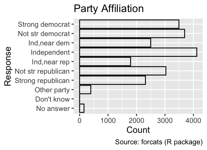
gg_gss<-ggplot(gss_cat, aes(y =partyid))+geom_bar(fill =NA, color ="black")+labs( x ="Count", y ="Response", fill ="Marital status", title ="Party Affiliation", caption ="Source: forcats (R package)")gg_gssgg_gss+scale_y_discrete( limits =c("Strong democrat", "Not str democrat", "Ind,near dem"))
Warning: Removed 11804 rows containing non-finite outside the scale range
(`stat_count()`).
9.2.2 Breaks
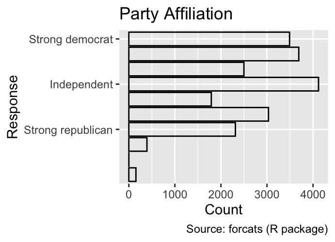
While the limits argument designates the possible values of the scale, the breaks argument specifies where labels and tick marks are placed. For example, the following plot shows the party affiliation of GSS participants, with the y-axis labels restricted to three categories:
Use the breaks argument to specify the values at which labels and tick marks are placed on a discrete scale.
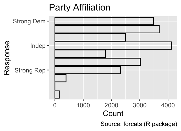
The labels argument allows you to specify the text displayed at each break. For instance, the code below abbreviates the labels of the y-axis tick marks:
Use the labels argument to define the text that appears at each break on a discrete scale.
This section explored how discrete scales can be customized using the scale_*_discrete() functions. These functions come equipped with limits, breaks, and labels arguments, each serving a distinct purpose:
The limits argument determines the potential values of the scale.
The breaks argument specifies label and tick-mark placement.
The labels argument defines the text that appears at each break.
9.3 ColorBrewer Palettes
As Section 8.1 illustrated, the default discrete palettes of ggplot2 employ colors that are evenly distributed in the HCL space. Although these palettes are adequate for exploratory data analysis, they may not always provide an optimal user experience. For example, they may not be ideal for colorblind readers or for print media. A more effective alternative is to select an appropriate palette from the array offered by the ColorBrewer project, which has been rigorously tested for human readability in cartographic applications. Most ColorBrewer palettes are designed to perform well across various media, such as paper and computer screens, and take into account color vision deficiencies. This section will introduce the three distinct types of ColorBrewer palettes: sequential (Section 9.3.1), diverging (Section 9.3.2), and qualitative (Section 9.3.3).
The three types of ColorBrewer palettes are sequential, diverging, and qualitative.
9.3.1 Sequential Palettes
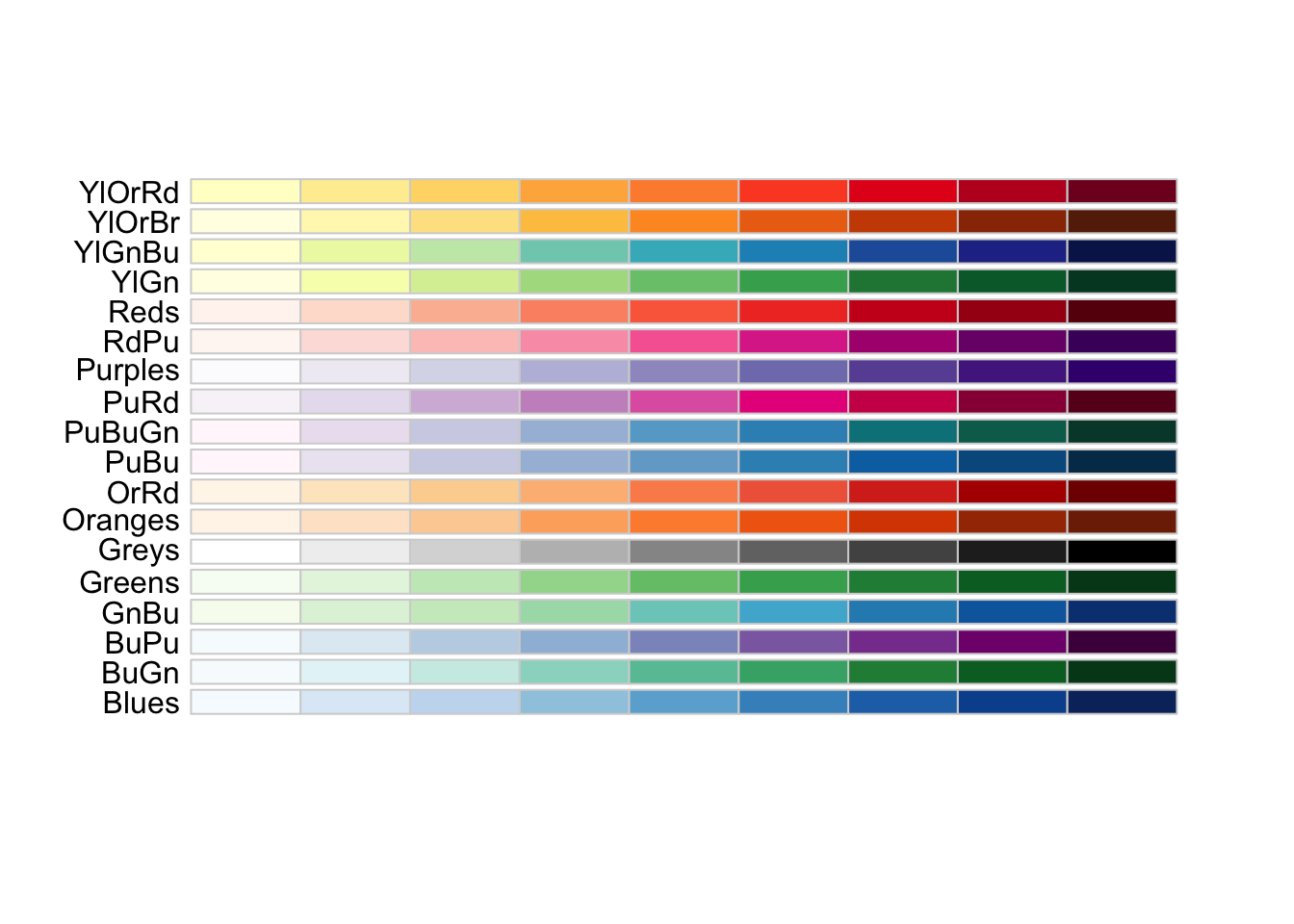
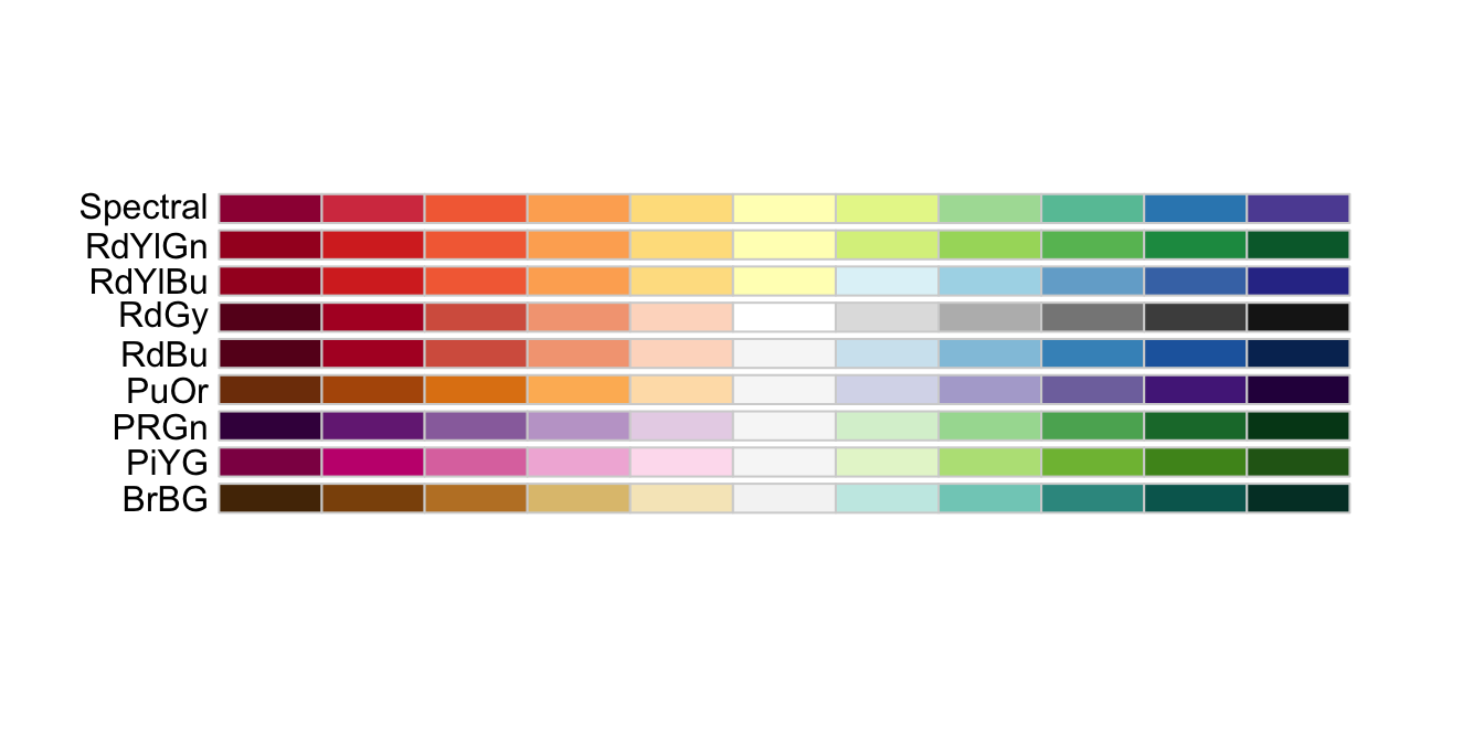
Sequential palettes are characterized by a gradation from a nearly white anchor color to colors of low luminance, encompassing only a limited range of hues. These palettes are particularly well-suited for representing non-negative data that are quantitative or ordinal in nature. You can view all available sequential palettes using the display.brewer.all() function from the RColorBrewer package.
Apply sequential palettes when representing non-negative quantitative or ordinal data.
Use display.brewer.all() from the RColorBrewer package to view all available sequential palettes.
To apply a sequential ColorBrewer scale to the interiors of objects, use the scale_fill_fermenter() function. Conversely, for coloring boundaries, you should use the scale_color_fermenter() function instead. When invoking these functions, the palette argument should be set to the desired palette name (e.g., "Blues").
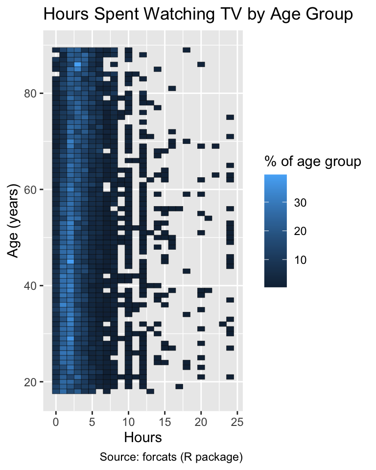
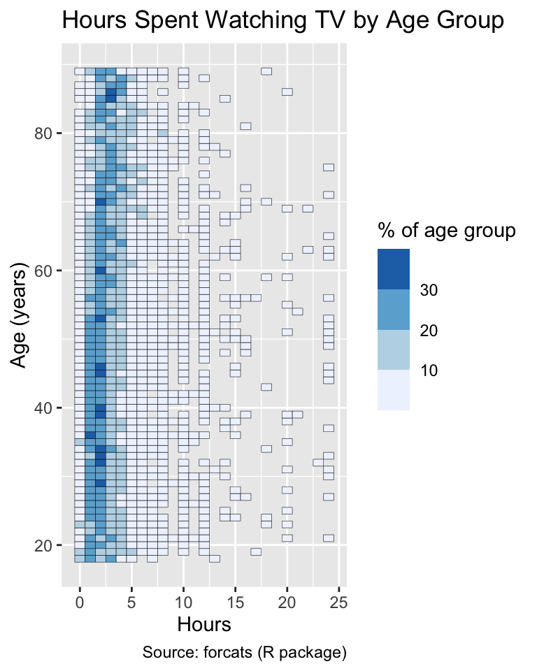
Sequential palettes are suitable for representing proportions or percentages within a group, as these quantities are always intensive and nonnegative. For example, the following code calculates the distribution of hours spent watching TV across different age groups of General Social Survey participants (see Section 8.1.2):
While the default palette of ggplot2 employs a continuum of colors, the scale_*_fermenter() functions adopt a discrete palette. Although discretization theoretically reduces the amount of information available from the originally continuous colors, human perception has limitations in distinguishing between colors that are too similar. Therefore, the discretization inherent in binned palettes may not significantly impact the accuracy of data interpretation. In fact, the increased contrast between different groups of data often facilitates the identification of overall patterns:
gg_tv<-ggplot(tv, aes(x =tvhours, y =age, fill =pct))+geom_tile(color ="black")+labs( x ="Hours", y ="Age (years)", fill ="% of age group", title ="Hours Spent Watching TV by Age Group", caption ="Source: forcats (R package)")gg_tvgg_tv+scale_fill_fermenter(palette ="Blues")
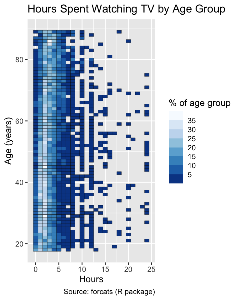
Ideally, discrete color palettes should consist of 4 to 9 bins, but the precise recommendations in the literature vary (see e.g., Declerq, 1995). If the default number of distinct colors produced by scale_*_fermenter() is deemed unsuitable, it can be adjusted using the n.breaks argument:
Use the n.breaks argument to modify the number of steps in a ColorBewer palette.
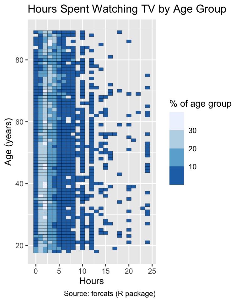
By default, ggplot2 represents small values with dark blue and large values with light blue. This default is suboptimal because most users intuitively interpret darker colors to represent larger values (Schiewe, 2024). A better approach is to invert the palette’s direction by setting the direction argument to 1:
Use the direction argument to choose the direction of a ColorBrewer palette such that lighter colors represent smaller values.
gg_tv+scale_fill_fermenter(palette ="Blues")gg_tv+scale_fill_fermenter(palette ="Blues", direction =1)
9.3.2 Diverging Palettes
Diverging palettes are designed for visualizing ordinal or quantitative data if they span from low to high values via a midpoint that can be regarded as neutral. These palettes are ideal for highlighting deviations from the midpoint in both directions. Here are the available diverging ColorBrewer palettes:
Apply diverging palettes when the data include both positive and negative values, with the lightest color representing zero.
Similar to sequential palettes, diverging palettes can be applied using the scale_*_fermenter() functions. The only difference is that the palette argument needs to correspond to the name of a diverging palette (e.g. "BrBG").
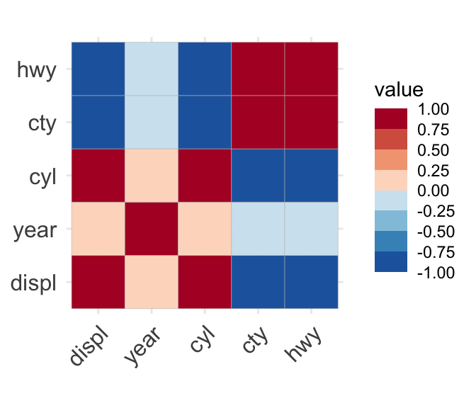
Diverging palettes should be used when the data include both positive and negative values, with the lightest color representing zero. For instance, the plot below illustrates the correlation coefficients of all numeric variables in the mpg tibble from the ggplot2 package, which comprises data on the fuel economy of 38 car models. The following variables are included:
displ: engine displacement, in liters
year: year of manufacture
cyl: number of cylinders
cty: city miles per gallon
hwy: highway miles per gallon
The plot suggests, for example, that highway miles per gallon tend to decrease as the number of cylinders increase. Conversely, the engine displacement tends to increase with the number of cylinders. The code employs the ggcorrplot() function from the ggcorrplot package:
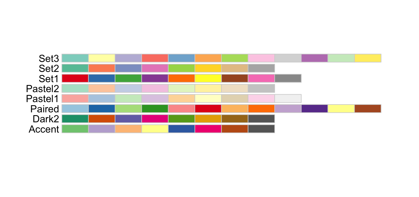
While sequential and diverging palettes are suitable when data are quantitative and ordinal, qualitative palettes are designed for unordered categorical data. These palettes employ distinct hues to differentiate between categories, with no inherent ordering. The following code displays all available qualitative ColorBrewer palettes:
Apply qualitative palettes when the data consist of unordered categorical variables.
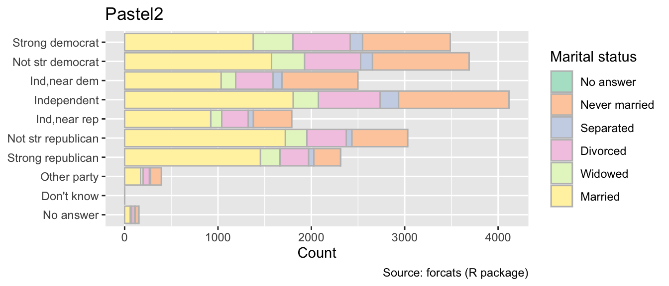
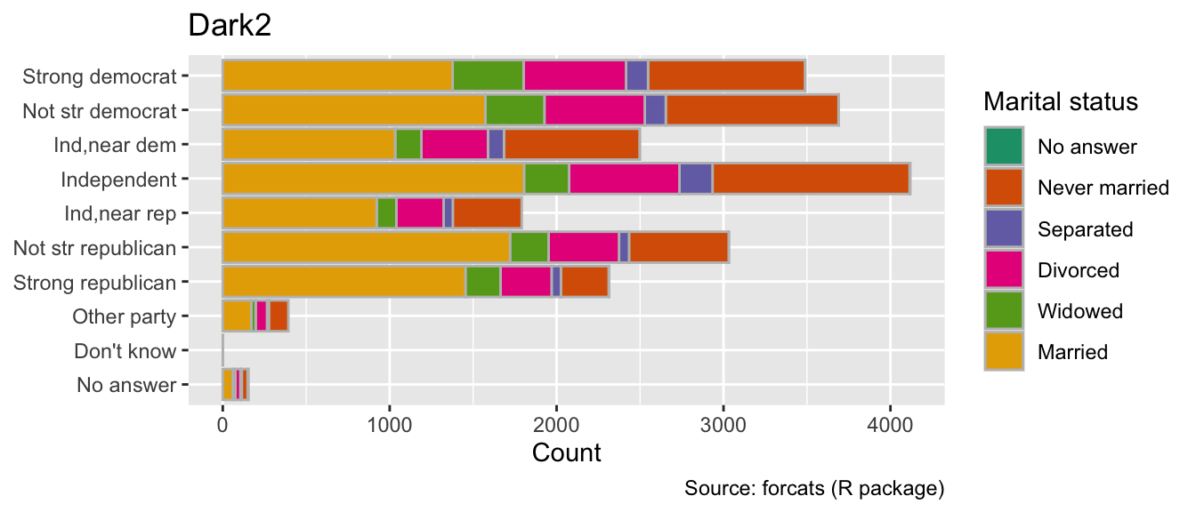
When coloring the interiors of objects, use the scale_fill_brewer() function with the palette argument equal to the desired palette name. For coloring boundaries, use the scale_color_brewer() function instead. In general, subdued palettes are more suitable for coloring the interiors of objects, while dark palettes are preferable for coloring points or lines (e.g., polygon boundaries). For example, the following code compares fill colors from the Pastel2 and Dark2 palettes. In my opinion, Pastel2 is more pleasant to the eye:
gg_gss<-ggplot(gss_cat, aes(y =partyid, fill =marital))+geom_bar(color ="grey")+labs( x ="Count", y =NULL, fill ="Marital status", caption ="Source: forcats (R package)")gg_gss+labs(title ="Pastel2")+scale_fill_brewer(palette ="Pastel2")gg_gss+labs(title ="Dark2")+scale_fill_brewer(palette ="Dark2")
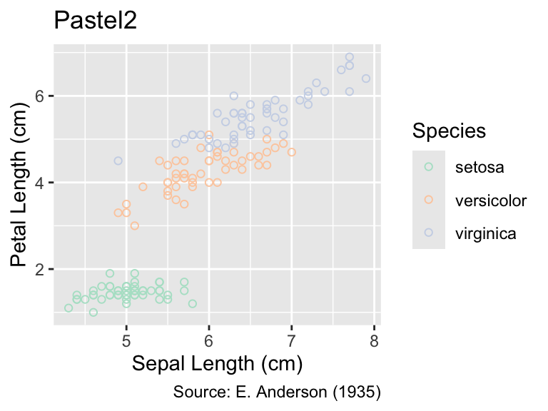
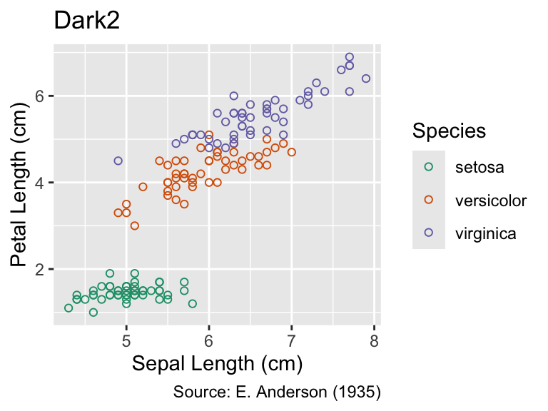
Conversely, the following plot uses the same palettes for points in the iris data set, colored according to species. The shape argument in the geom_point() function is set to 1 to display open circles. A list of point symbols and their corresponding integer code is available at ?points. In this case, the Pastel2 palette is too subtle in my opinion, making it difficult to discern the point locations. Dark2 is more suitable for this purpose:
gg_iris<-ggplot(iris, aes(Sepal.Length, Petal.Length, color =Species))+geom_point(shape =1)+labs( x ="Sepal Length (cm)", y ="Petal Length (cm)", caption ="Source: E. Anderson (1935)")gg_iris+labs(title ="Pastel2")+scale_color_brewer(palette ="Pastel2")gg_iris+labs(title ="Dark2")+scale_color_brewer(palette ="Dark2")
9.3.4 Section Summary: ColorBrewer Palettes
The ColorBrewer palettes offer a superior alternative to ggplot2’s default color schemes, enhancing the visual appeal and readability of plots. The scale_*_fermenter() functions from the ggplot2 package provide an easy interface to apply sequential and diverging ColorBrewer palettes to plots, whereas the scale_*_brewer() functions should be used to select qualitative palettes. While the strategic use of colors can significantly enhance the aesthetic and interpretive quality of plots, it is important to use them judiciously. In particular, remember that color should be used only for intensive data.
9.4 Scales for the Size Aesthetic
Size can refer to either the area or a linear dimension (e.g., the radius) of an object. When mapping a statistical variable to the size aesthetic, it is important to choose the appropriate geometric interpretation. Section 9.4.1 will demonstrate how to achieve area-proportional size scaling, which is typically more intuitive than scaling in proportion to a length scale. However, in rare cases, it may be preferable to scale the size aesthetic by the symbol’s linear dimension rather than by its area; this alternative is discussed in Section 9.4.2.
Regardless of the chosen scaling method, remember from Section 8.2 that the size aesthetic should be mapped exclusively to extensive variables, ensuring consistency with the additive and nonnegative perception of this visual stimulus.
9.4.1 Scaling by Area
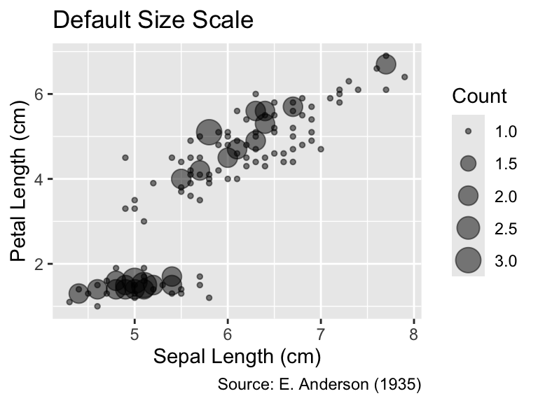
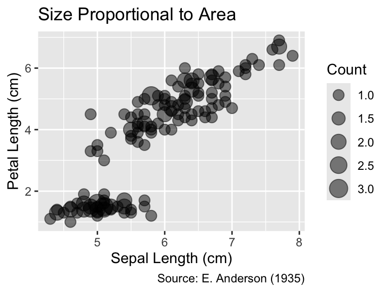
When employing size as an aesthetic—either explicitly through the aes() function or implicitly, as done by geom_count()—ggplot2 chooses symbol areas that increase with the data value, albeit not necessarily proportionally to it. For instance, in the left plot presented below, a count of 1 is represented by a circle whose area is significantly smaller than half the area of the circle depicting a count of 2. To ensure that the area of the symbols is proportional to the data values, you can use the scale_size_area() function, as illustrated by the right plot. Generally, it is good practice to invoke scale_size_area() when using the size aesthetic to adhere to Tufte’s (1983) principle of graphical integrity (see Section 1.2.1).
The default size scale in ggplot2 does not proportionally scale areas or radii to the data values. It is usually advisable to invoke scale_size_area() to achieve proper area scaling.
gg_iris<-ggplot(iris, aes(Sepal.Length, Petal.Length))+geom_count(alpha =0.5)+labs( x ="Sepal Length (cm)", y ="Petal Length (cm)", size ="Count", caption ="Source: E. Anderson (1935)")gg_iris+labs(title ="Default Size Scale")gg_iris+scale_size_area()+labs(title ="Size Proportional to Area")
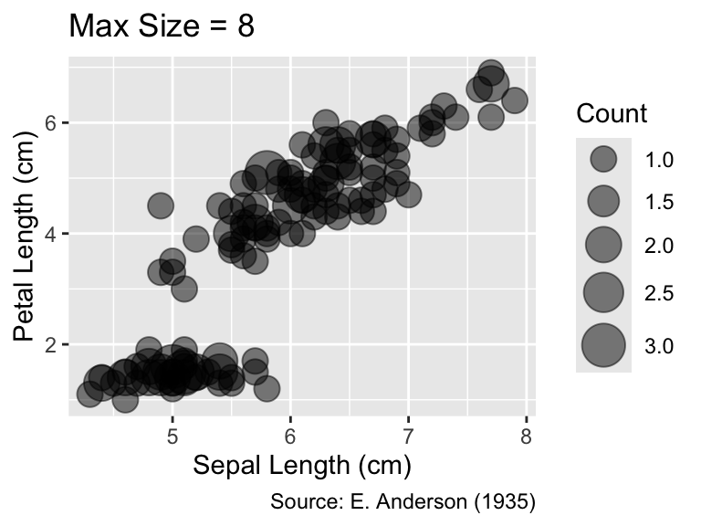
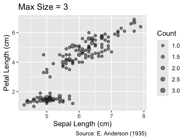
An important parameter of scale_size_area() is max_size, which determines the maximum size of the symbols. The default value is 6. The following plots illustrate the effect of changing max_size to either 8 or 3. In this example, the smaller value is preferable because it reduces symbol overlaps:
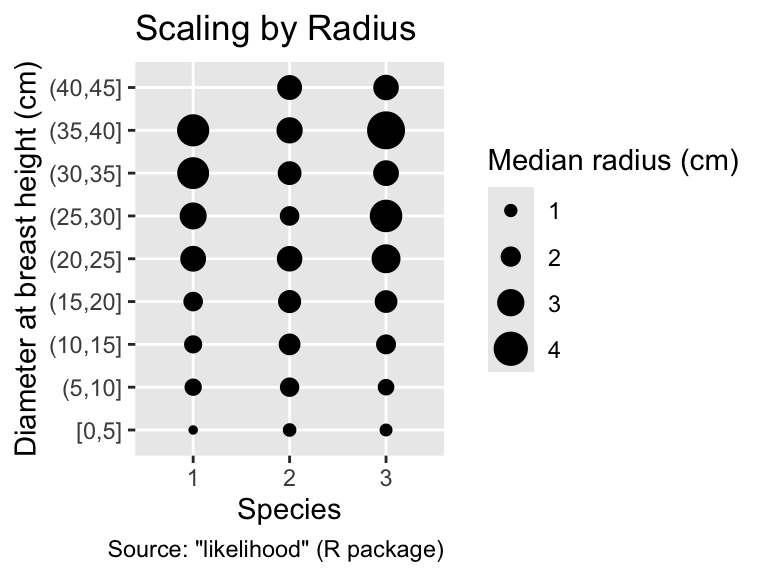
In most applications, the size aesthetic should be proportional to the area of the symbols. However, there are exceptions where it is more appropriate to scale size in proportion to the linear extent, such as the radius, rather than the area. For instance, the crown_rad data set from the likelihood package contains a Radius column that represents the crown radius of trees:
To visualize the data, let us first bin the observations based on the diameter at breast hide (DBH) in intervals of length 5. Subsequently, the median radius for each bin and species can be calculated:
crown_rad_summarised<-crown_rad|>mutate( species =factor(Species), bin =cut_interval(DBH, length =5))|>summarise(median_radius =median(Radius), .by =c(bin, species))head(crown_rad_summarised)
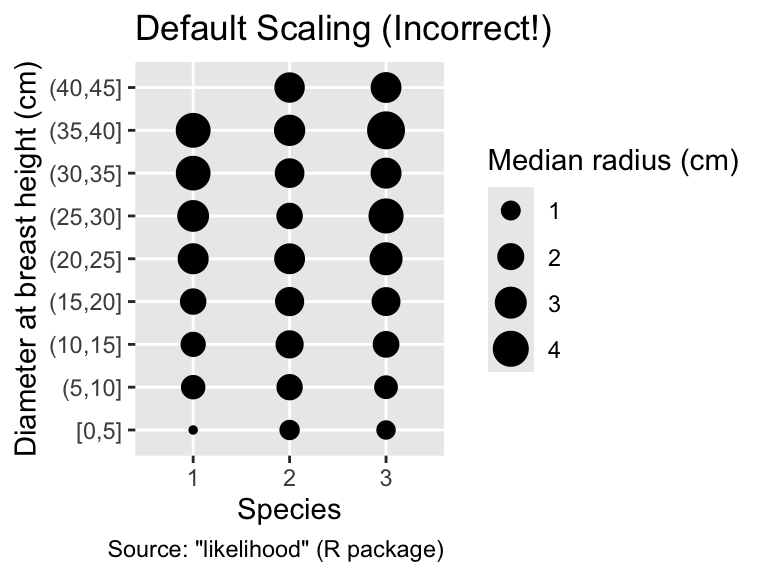
Finally, to accurately represent the median crown radius, the scale_radius() function can be invoked. In contrast, ggplot2’s default scaling misrepresents the data, as the symbols exhibit less size variation than the actual physical crown radii do:
Use scale_radius() when representing physical radii of objects.
g_crown_rad<-ggplot(crown_rad_summarised, aes(species, bin, size =median_radius))+geom_point()+labs( x ="Species", y ="Diameter at breast height (cm)", size ="Median radius (cm)", caption ='Source: "likelihood" (R package)')g_crown_rad+labs(title ="Scaling by Radius")+scale_radius()g_crown_rad+labs(title ="Default Scaling (Incorrect!)")
9.4.3 Section Summary: Scales for the Size Aesthetic
This section has highlighted the importance of the size aesthetic in data visualization, emphasizing that symbol size can be interpreted in terms of area or linear extent. When utilizing ggplot2’s default scales, neither the areas nor the radii of symbols scale strictly in proportion to the data values. Therefore, it is generally recommended to employ the scale_size_area() function to ensure a proportional relationship between areas and data values for most applications. In the less common scenarios where data values specifically pertain to physical radii, the scale_radius() function is the appropriate choice to accurately represent the data.
9.5 Conclusion
This chapter has explored various aspects of manipulating ggplot2 scales. You have learned how to tailor limits, breaks, and labels for both continuous and discrete scales. Moreover, this chapter has made you aware of the nuances of working with color and size scales. Thoughtful applications of these scales are required to ensure the graphical integrity of data visualization.
Declerq, F.A.N. (1995) “Choropleth map accuracy and the number of class intervals,” in Proceedings of the 16th international cartographic conference. Barcelona: International Cartographic Association, pp. 918–922.
Schiewe, J. (2024) “Dark-is-More Bias Also in Dark Mode? Perception of Colours in Choropleth Maps in Dark Mode,”KN - Journal of Cartography and Geographic Information, 74(2), pp. 171–180. Available at: https://doi.org/10.1007/s42489-024-00171-z.
Tufte, E.R. (1983) The visual display of quantitative information. Cheshire: Graphics Press.