c(31, -50, 9.3, 29, -4.483, 93)[1] 31.000 -50.000 9.300 29.000 -4.483 93.000This chapter aims to equip you with essential R skills. By the end, you will be able to:
The focus is on those aspects of R that are most relevant for data visualization. Consequently, the chapter does not aspire to provide a comprehensive introduction to R. For a more detailed introduction, I recommend reading An Introduction to R by Venables, Smith and the R Core Team (2025).
R vectors encapsulate a combination of elements, all belonging to the same class; for example, it is possible that every element is a number or every element is a character string. By the conclusion of this chapter, you will have learned how to create vectors, assign them to variables (Section 4.1.1), distinguish between the most important vector classes (Section 4.1.2), and extract subsets from vectors (Section 4.1.3).
R provides various tools for creating vectors comprising one or more elements. The most general method is provided by the c() function. which combines the elements listed inside the parentheses into a vector. Here is an example of a numeric vector. The output line begins with [1] to indicate that the subsequently printed value, 31, is the first element in the vector:
Use c() to combine elements into a vector.
c(31, -50, 9.3, 29, -4.483, 93)[1] 31.000 -50.000 9.300 29.000 -4.483 93.000If values in an R object (e.g., a vector) are referred to multiple times in a calculation, it can be tedious to type all the elements repeatedly. Instead, it is more convenient to save the object in a variable and refer to it by name. In the following example, R assigns a vector to a variable named v:
Use <- to assign an R object to a variable.
v <- c(31, -50, 9.3, 29, -4.483, 93)The symbol <-, composed of a greater-than sign and a hyphen, is called the assignment operator. It is often pronounced as “gets” because, for example in this case, v gets assigned the combination of numbers on the right-hand side.
After a variable has been defined, its content can be viewed by typing its name in the console and pressing the return key:
Enter the name of a variable in the console to view its content.
v[1] 31.000 -50.000 9.300 29.000 -4.483 93.000Vectors in R can belong to different classes depending on the type of data they store. The following sections will introduce the most important classes: numeric (Section 4.1.2.1), character (Section 4.1.2.2), and logical vectors (Section 4.1.2.3). Finally, Section 4.1.2.4 will demonstrate that R converts all elements to the same class if a user attempts to combine different classes into a vector.
Numeric vectors can store positive and negative numbers, including floating-point values. The vector v, as defined in Section 4.1.1, exemplifies a numeric vector, as can be confirmed using the class() function:
Use class() to retrieve the class of a vector.
class(v)[1] "numeric"The is.numeric() function can be used to check if a vector is numeric:
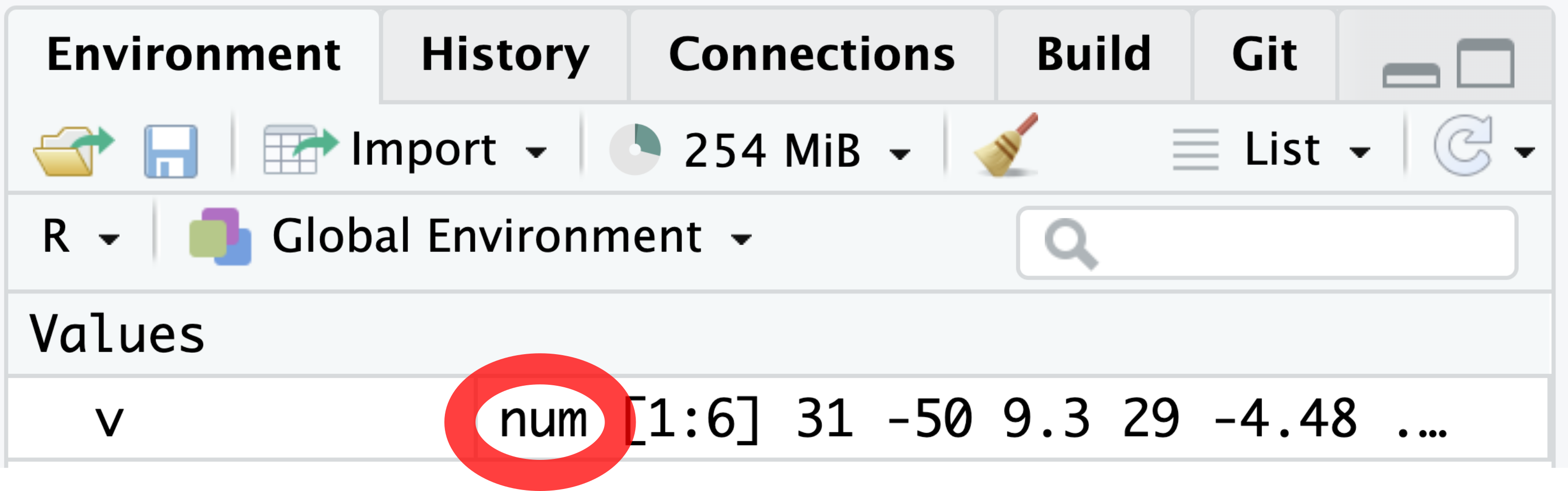
is.numeric(v)[1] TRUEAn alternative method to confirm that v is a numeric vector is by inspecting the Environment tab, located in the top right of the RStudio window. The Environment tab denotes the numeric class as “num” (Figure 4.1).
R provides a set of basic arithmetic operators for performing calculations with numeric vectors, as shown in Table 4.1.
%/%) has a forward slash (/) between the percent signs, whereas the modulo operator (%%) does not contain a forward slash.
| Operator | Description |
|---|---|
x + y |
Sum of x and y
|
x - y |
y subtracted from x
|
x * y |
x multiplied by y
|
x / y |
x divided by y
|
x^y or x**y
|
x raised to the power y
|
x %/% y |
Integer division. Example: 7 %/% 3 returns 2. |
x %% y |
x modulo y (i.e., remainder after integer division of x by y). Example: 7 %% 3 returns 1. |
All these arithmetic operations are carried out element-wise. For example, when v and 2 in the following code chunk are added together using the + operator, then the n-th element of the output is the sum of the n-th elements of v and w:
Arithmetic operations on vectors are performed element-wise.
w <- c(4, 3, 1, 2, 6, 5)
v + w
[1] 35.000 -47.000 10.300 31.000 1.517 98.000When one of the operands in an arithmetic operation is a vector of length 1, then this operand is applied to all elements of the other operand. For instance, the following code subtracts 2 from each element of w:
w - 2[1] 2 1 -1 0 4 3Besides basic arithmetic operators, R also possesses various functions for summarizing numeric vectors. For instance, the sum() function, when applied to a vector, adds up all its values:
sum(w)[1] 21Additional functions summarizing a vector with a single number include mean(), min(), and max().
While the c() function serves as the most general tool for creating vectors, R offers shortcuts for creating numeric sequences. When consecutive numbers differ by +1 or -1, the colon operator (:) provides a convenient shortcut:
Use : to create sequences of consecutive numbers differing by +1 or -1.
3:10[1] 3 4 5 6 7 8 9 103.5:-5.5 [1] 3.5 2.5 1.5 0.5 -0.5 -1.5 -2.5 -3.5 -4.5 -5.5For more general sequences, the seq() function can be used, which typically requires three numeric arguments, named from, to, and by. The first two numbers denote the start and end points of the sequence, and the third argument is the step size:
Use seq() to create sequences of numbers with a specified arbitrary step size.
seq(from = 0.5, to = 20.1, by = 0.4) [1] 0.5 0.9 1.3 1.7 2.1 2.5 2.9 3.3 3.7 4.1 4.5 4.9 5.3 5.7 6.1
[16] 6.5 6.9 7.3 7.7 8.1 8.5 8.9 9.3 9.7 10.1 10.5 10.9 11.3 11.7 12.1
[31] 12.5 12.9 13.3 13.7 14.1 14.5 14.9 15.3 15.7 16.1 16.5 16.9 17.3 17.7 18.1
[46] 18.5 18.9 19.3 19.7 20.1The number enclosed in square brackets at the start of an output line indicates the position of the following printed value in the vector. For example, [16] indicates that 6.5 is the value of the 16th element in the vector.
Vectors can also store non-numeric data, such as character strings. In computer terminology, a character string is a combination of letters, numbers, and special symbols that is interpreted as a text object. In R, character strings must be enclosed in quotation marks, for example:
Character strings must be enclosed in quotation marks.
compass <- c("North", "East", "South", "West")The class of a vector containing character strings is character:
class(compass)[1] "character"The is.character() function can be used to determine whether a vector belongs to the character class:
is.character(compass)[1] TRUEIn the Environment tab, the character class is abbreviated as “chr” (Figure 4.2).
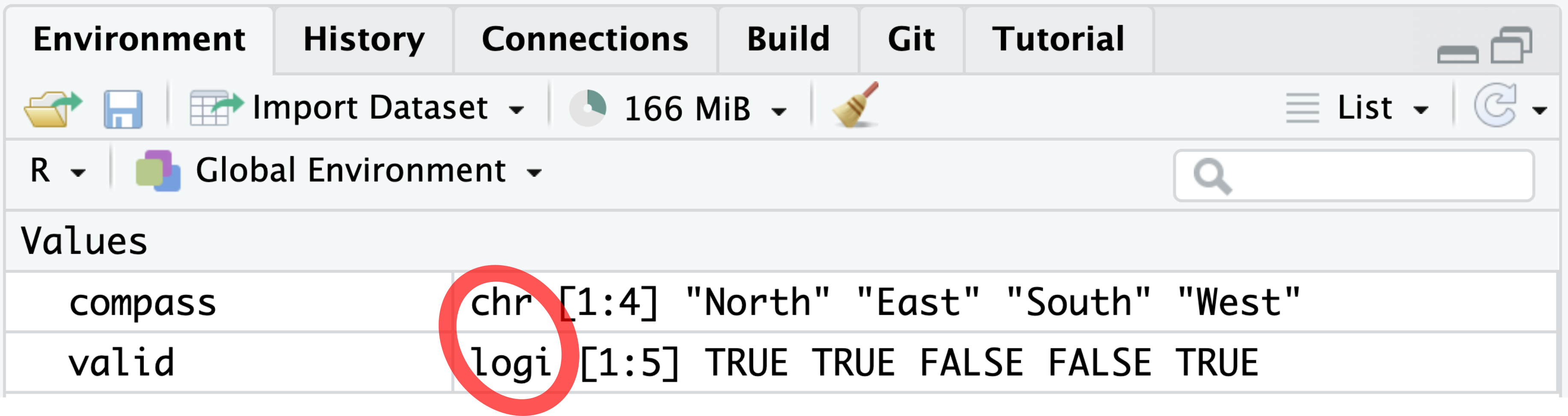
compass and valid belong to the character and logical classes, respectively.
A logical vector, such as valid in the code chunk below, consists of elements that are either TRUE or FALSE:1
Logical vectors can contain only TRUE and FALSE values.
Please note that TRUE and FALSE are not enclosed in quotation marks. Otherwise, R would interpret "TRUE" and "FALSE" as character strings instead of logical values:
class("TRUE")[1] "character"The is.logical() function can be applied to test whether a vector contains logical values:
In the Environment tab, the class name logical is abbreviated as “logi” (Figure 4.2).
A common question arising in data analysis is whether all or at least some elements of a logical vector are TRUE. In R, this question can be answered using the all() function, which returns TRUE if and only if all elements in the argument are TRUE. For example, valid contains FALSE elements; hence, all(valid) returns FALSE:
all() returns TRUE if and only if all elements in the argument are TRUE.
all(valid)[1] FALSELogical vectors often arise from comparisons between two other vectors. For example, the following code compares the elements of x and y, returning a logical vector that indicates whether the corresponding elements in x are equal to those in y:
The equality operator == is one of several comparison operators available in R. Table 4.2 lists other common comparison operators. If applied to character vectors, its elements are compared alphabetically.
| Operator | Description: TRUE if and only if … |
|---|---|
x == y |
x equals y
|
x != y |
x does not equal y
|
x < y |
x is less than y
|
x > y |
x is greater than y
|
x <= y |
x is less than or equal to y
|
x >= y |
x is greater than or equal to y
|
x %in% y |
x is an element in y
|
Another common operation resulting in a logical vector is the negation of another logical vector (i.e., converting TRUE into FALSE and vice versa). Negation is represented in R by the exclamation mark (!). For example, !valid indicates whether an element is invalid:
Use ! for NOT operations.
!valid[1] FALSE FALSE TRUE TRUE FALSEFurther logical operations include & (AND) and | (OR). For example, suppose we are given a logical vector named credible in addition to valid:
The logical operators & and | perform AND and OR operations, respectively.
credible <- c(TRUE, FALSE, TRUE, FALSE, FALSE)The combination valid & credible returns a logical vector that is TRUE if and only if both valid and credible are TRUE:
valid & credible[1] TRUE FALSE FALSE FALSE FALSEIn contrast, the combination valid | credible produces a logical vector that is TRUE if at least one of the two vectors is TRUE:
valid | credible[1] TRUE TRUE TRUE FALSE TRUEAn important property of a vector is that all its elements must share the same class. If the input elements are of different classes, R automatically converts the data types such that this property remains valid. R does not warn the user when performing this conversion. However, in most cases, it is the result of an unintentional error by the user.
It is impossible to mix different classes in a vector.
The following example demonstrates that combining a number and a character string produces a character vector:
It is evident from the console output that 1 has become a character string because it is enclosed in quotation marks:
mix_attempt[1] "1" "a"Please note that it is impossible to perform any arithmetic operation, such as addition, on character strings:
"1" + "1"Error in "1" + "1": non-numeric argument to binary operatorOnce a vector has been created, it is often necessary to extract specific elements from it. For example, you may want to extract the first element or obtain a subset containing only the last few elements. The most common method for element extraction is to insert the target indices inside square brackets. For example, the following code extracts the first element and the third to sixth elements, respectively, from s:
Use square brackets ([]) to extract elements from a vector.
When inspecting a vector during exploratory data analysis, it is often useful to extract the first few elements. The head() function can be used for this purpose. By default, it returns the first six elements of a vector:
head(s)[1] 0.5 0.9 1.3 1.7 2.1 2.5Similarly, the tail() function retrieves the last six elements:
tail(s)[1] 18.1 18.5 18.9 19.3 19.7 20.1To extract all unique values in a vector, eliminating any repetition, use unique():
The unique() function returns all unique values in a vector.
This section introduced vectors, the fundamental building blocks of R. Below are the key takeaways:
c() function combines elements into a vector.numeric, character, and logical.[]).In statistical samples, data points are often unavailable for various reasons, such as equipment failure or non-responses in surveys. To represent such missing data, R uses the special value NA and allows vectors of all classes to contain NA elements. Please note that NA is not enclosed in quotation marks because "NA" would represent a character string composed of the letters N and A instead of a missing value. Here are examples of vectors containing NA:
NA represents unavailable data.
Most operations and functions produce NA when at least one of their arguments is NA. For instance, the fourth element of the following vector is NA because NA + 2 equals NA:
Operations involving NA usually result in NA.
nums + 2[1] 3 4 5 NA 7 8At first glance, it might seem reasonable to identify NA values in nums using the expression nums == NA. However, the output from nums == NA does not answer whether an element is NA. Instead, all elements of nums == NA are NA themselves:
nums == NA[1] NA NA NA NA NA NATo verify that an element equals NA, the function is.na() should be used instead:
Never use == NA. Use is.na() instead.
is.na(nums)[1] FALSE FALSE FALSE TRUE FALSE FALSEConsistent with the rule that operations involving NA result in NA, functions for summary statistics—such as sum(), mean(), min(), and max()—also return NA if any element in the input equals NA, for example:
mean(nums)[1] NAOn the one hand, returning NA is sensible because the true mean is indeed unknown when there are unavailable data points. However, it is often reasonable to compute the mean from the sample of non-NA values. In such cases, na.rm = TRUE can be added to the argument list of the mean() function:
mean(nums, na.rm = TRUE)[1] 3.4Like mean(), many other R summary statistics functions (e.g., sum(), min(), and max()) also accept the optional na.rm = TRUE argument. It is advisable to check the R documentation of the respective function for clarification.
Include na.rm = TRUE to remove NA from summary statistics computation.
Thoughtful handling of missing values ensures that data analysis and visualization remain accurate and meaningful. By providing NA as a unified missing-value alongside dedicated tools such as is.na() and the na.rm argument, R offers principled support for this task.
Learning a programming language can be intimidating, and R is no exception. However, fear not, as there is an abundance of resources available to assist you when working with R. This section will explore some of the most frequently used references that even experienced R programmers consult for guidance. Section 4.3.1 will introduce R’s built-in documentation, which is the main reference for functions and built-in data sets, conveniently accessible from the console through the question-mark operator (?). Afterward, Section 4.3.2 will discuss strategies for seeking help on the World Wide Web, from harnessing the power of search engines and artificial intelligence to posting questions on public message boards.
The primary source of information about R is its built-in documentation. Almost all R functions and built-in data sets are accompanied by a corresponding help page. The help page can be accessed by typing a question mark followed by the name of the R object to be looked up. For example, the following command opens the help page for the seq() function:
Use ? followed by the name of the function or data set to open the respective help page.
?seqWhen using RStudio, the help page will open in the bottom right pane. Let us explore the information provided in this pane.
Each help page begins with a concise description (Figure 4.3), enabling the user to judge quickly if the described function or data set is relevant to their needs.
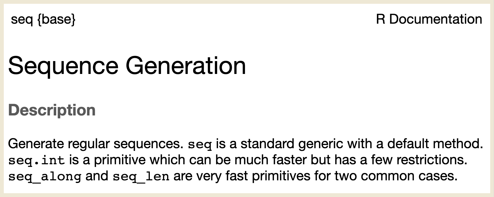
seq() function provides a concise description of the function’s purpose.
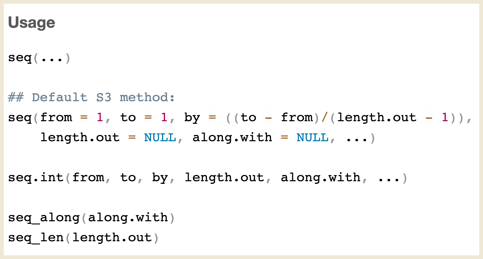
The second section on most help pages is dedicated to “Usage” (Figure 4.4). It provides information on the arguments that the function accepts. For instance, the seq() function can take arguments such as from, to, and by. Additionally, the “Usage” section often includes a list of related functions. In this example, seq.int(), seq_along(), and seq_len() are listed because they are connected to the concept of sequence generation.
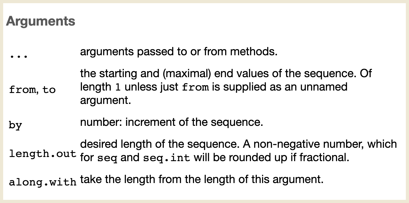
The third section, titled “Arguments,” provides further details about the arguments, including their classes and their respective meanings (Figure 4.5).
The fourth section, “Details,” provides additional context (Figure 4.6). For instance, in the case of seq(), the “Details” section clarifies that no infinite or missing numeric values should be used. Although parts of the description may appear cryptic at first, they will become clearer as you gain more experience with R.
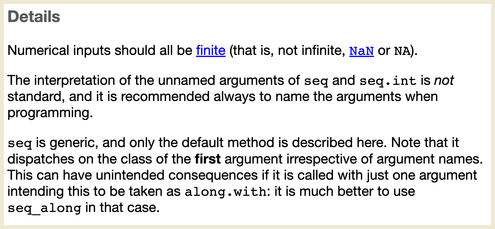
seq(). For this and other functions, the “Details” section delves into more technical depth than the preceding sections.
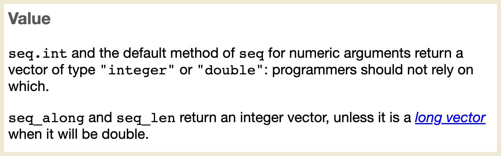
The fifth section, “Value,” specifies the data type and structure of the function’s output. For instance, the return value of seq() is a numeric vector that may contain integers or double-precision floating-point numbers (Figure 4.7).
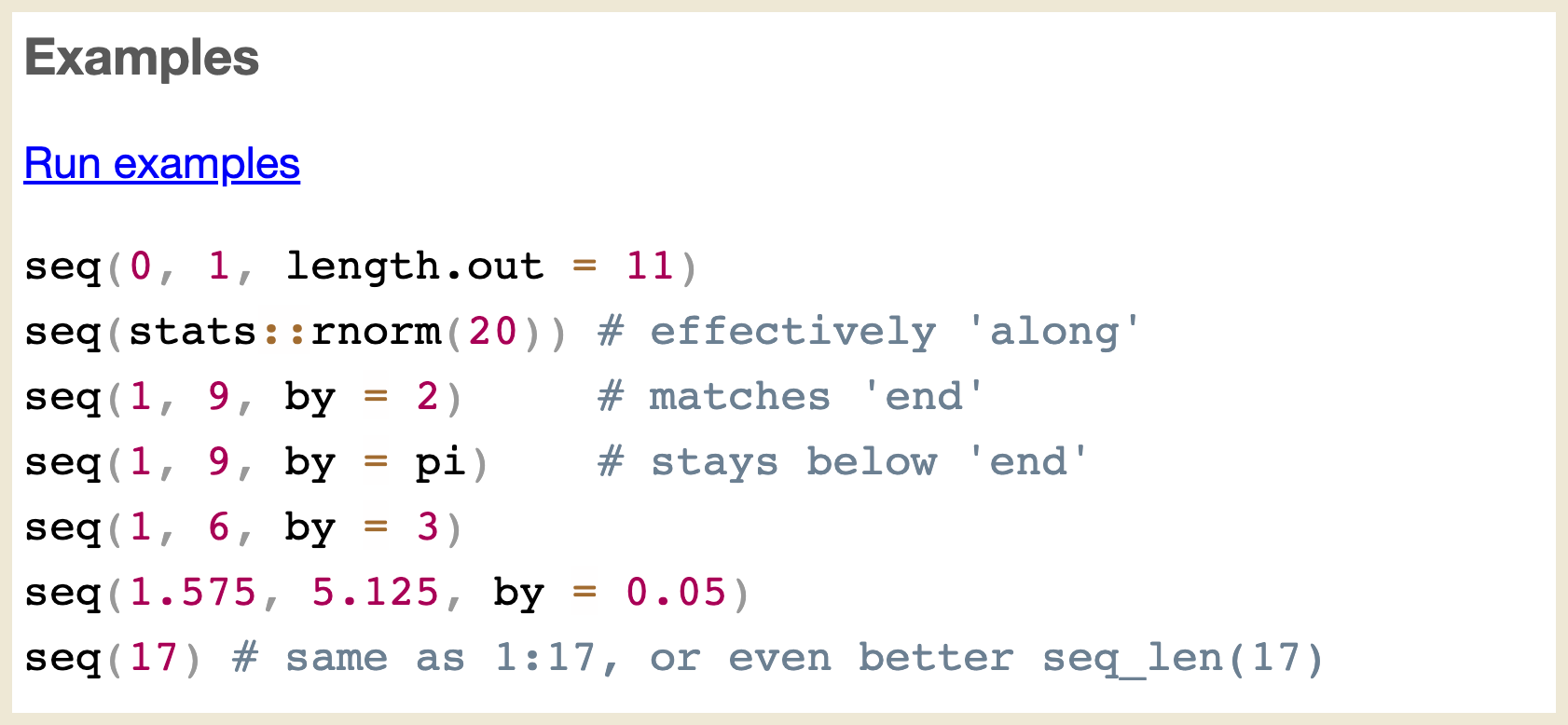
An example often explains more than many words. For this reason, almost every built-in help document in R ends with examples (Figure 4.8). You can copy and paste individual lines to the console, or you can run all examples by clicking on the “Run examples” button.
One disadvantage of the ? operator is that the name of the function or data set needs to be already known before searching for it. When you do not know the precise name yet, you can use the ?? operator. If the search term contains a space, quotation marks around the search term are required:
Use ?? followed by the search term to find all help pages that contain this word or phrase.
??variance
??"standard deviation"
After entering these commands, RStudio lists all pages in the built-in documentation that contain the phrase between the quotation marks.
For broader searches, you can resort to search engines, such as Google, or generative artificial intelligence, such as ChatGPT. These tools are especially effective when your code produces a cryptic error message. Copying and pasting the error message into a search engine or chatbot often leads to websites that explain and solve the error. Including “R” in the query string or prompt increases the probability of obtaining relevant search results.
Copying and pasting an error message into a search engine often helps to resolve the issue.
If you still cannot find a solution, consider posting a question on public message boards. Among the relevant user forums are R-help, the Posit community portal, and Stack Overflow. For questions on R programming, R-help is a free, general mailing list, maintaining a message board for its subscribers. However, questions specifically about RStudio are more likely to be answered on the Posit community portal, supported by the RStudio developers. Stack Overflow is a broader forum, not dedicated solely to R or RStudio but nevertheless visited by many active R users eager to share their knowledge.
The main forums for seeking assistance are R-help, the Posit community portal, and Stack Overflow.
When posting a question on a public message board, it is important to provide a minimal example that enables others to reproduce the error on their own computer and provide meaningful advice. It takes a little bit of practice to ask good questions on public message boards, but the responses are often insightful and surprisingly quick.
Although R has its idiosyncrasies (Burns, 2011), its extensive built-in documentation and vibrant community are invaluable resources. When you run into an issue, use ? or ?? in the console, Internet Search Engines, generative artificial intelligence, or consult online forums. Assistance is usually just a command or a click away.
The base installation of R contains an extensive selection of built-in functions and data sets. In practice, however, you will still often encounter challenges that are difficult to solve only with the functions and data sets available in R’s base installation. When you encounter such a challenge, you may find it reassuring that the R community is big and diverse; therefore, somebody else has probably already faced a similar challenge. Furthermore, many R community members contribute additional functions and data sets to solve problems outside the scope of R’s base installation. Such additional collections of code are called packages.
R’s official package repository is known as the Comprehensive R Archive Network (CRAN). Currently, there are more than 20,000 packages available on CRAN. When you face a challenging task, it is worth checking whether one of these packages can assist you.
This section will show how to integrate CRAN packages into your workflow. In Section 4.4.1, you will learn how to install packages, and Section 4.4.2 will focus on loading their content.
Packages are collections of functions and data sets that extend R’s capabilities.
The names of all packages currently loaded can be obtained using the .packages() function:
The output above includes the typical preloaded packages at the start of an R session. These packages contain most of the functions encountered in everyday use. After loading new packages, you will see additional elements in the output.
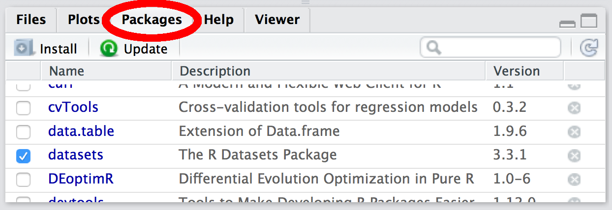
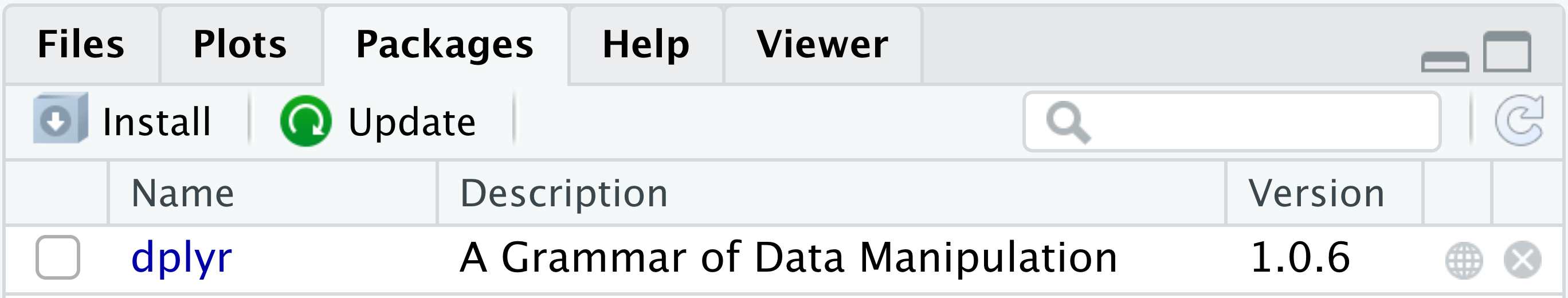
Alternatively, you can inspect the Packages tab in the lower right RStudio pane (Figure 4.9). Every package that is marked by a tick is currently loaded in the active R session. Unticked packages are installed but not loaded. The distinction between installation and loading is important, as you will see shortly.
If you want to check whether a specific package is installed, you can either scroll through the list in the Packages tab or look through the output of the following command:
In this book, we will work extensively with the dplyr package. Let us check whether dplyr is listed in the packages tab:
find.package("dplyr")If this command generated an error, then dplyr is not installed on your computer. Otherwise, please remove the dplyr package temporarily for demonstration purposes. There are two ways to remove a package:
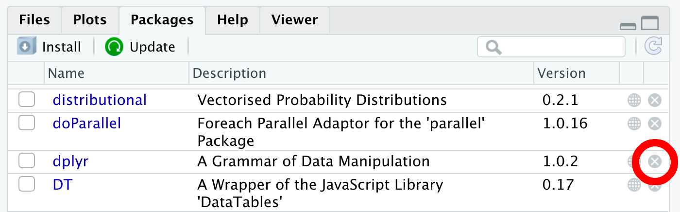
Run the function remove.packages().
remove.packages("dplyr")Click the \(\otimes\) button to the right of “dplyr” in the packages tab (Figure 4.10).
To install a package, you can run the install.packages() function while being connected to the internet:
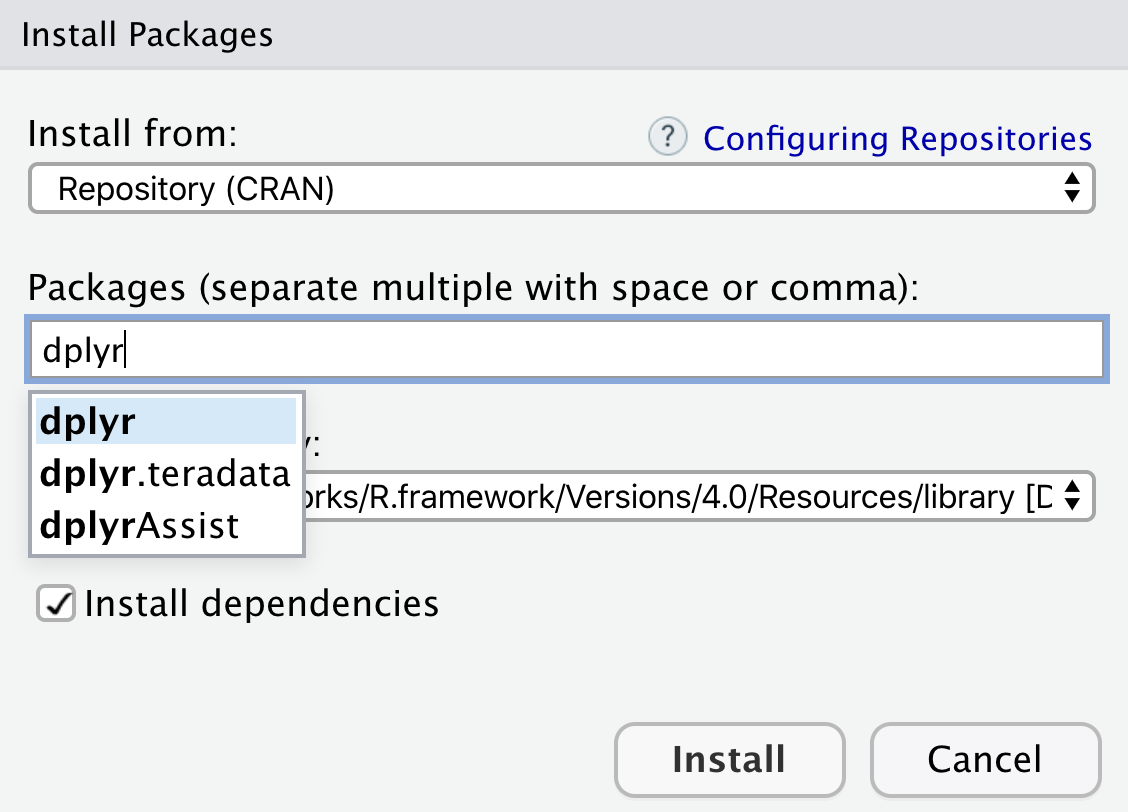
install.packages("dplyr")Alternatively, you can click the “Install” button in the Packages tab. It opens a dialog box where you can type the name of the package you want to install (Figure 4.11). While you are typing, RStudio will try to automatically complete the package name, which conveniently reduces the probability of typos. Then, click “Install.” The download and installation should only take a few seconds.
Use either install.packages() or the Packages tab to install packages.
The dplyr package contains a variety of functions and data sets. These are listed in the package documentation, which can be viewed in the Help tab, located in the lower right RStudio pane, after running the following command:
help(package = "dplyr")One of the data sets in the dplyr package is starwars, which contains information about the characters in the Star Wars film series. Let us try to take a look at the data by typing starwars in the console:
starwarsError: object 'starwars' not foundWhy can R not find starwars? Has the necessary package not just been installed?
Yes, but installing a package is not the same as loading it. When you installed the package, you saved the data on your computer, but the data are not automatically loaded into the current R session.
You can load the content of a package using either the double-colon operator (::), as explained in Section 4.4.2.1, or the library() function, as detailed in Section 4.4.2.2.
The double-colon operator (::) provides access to objects in a specific package. The package needs to be named on the left side of the operator, and the requested function or data set in the package must be specified on the right side. For example, to access the starwars data set in the dplyr package, you can type:
The :: operator provides access to objects in a specific package.
dplyr::starwars# A tibble: 87 × 14
name height mass hair_color skin_color eye_color birth_year sex gender
<chr> <int> <dbl> <chr> <chr> <chr> <dbl> <chr> <chr>
1 Luke Sk… 172 77 blond fair blue 19 male mascu…
2 C-3PO 167 75 <NA> gold yellow 112 none mascu…
3 R2-D2 96 32 <NA> white, bl… red 33 none mascu…
4 Darth V… 202 136 none white yellow 41.9 male mascu…
5 Leia Or… 150 49 brown light brown 19 fema… femin…
6 Owen La… 178 120 brown, gr… light blue 52 male mascu…
7 Beru Wh… 165 75 brown light blue 47 fema… femin…
8 R5-D4 97 32 <NA> white, red red NA none mascu…
9 Biggs D… 183 84 black light brown 24 male mascu…
10 Obi-Wan… 182 77 auburn, w… fair blue-gray 57 male mascu…
# ℹ 77 more rows
# ℹ 5 more variables: homeworld <chr>, species <chr>, films <list>,
# vehicles <list>, starships <list>Specifying the package with the double-colon operator has the advantage that it is guaranteed to retrieve the correct object if there is a naming conflict (i.e., if another package happens to contain another object with the same name). One disadvantage of using the double-colon operator is the need to repeatedly type dplyr:: if your code relies on multiple dplyr functions or data sets.
library()
The library() function provides an alternative to the double-colon operator for loading the content of a package. The package name is passed as an argument and does not need to be enclosed in quotes:
Use library() to load a package for the entire duration of an R session.
Attaching package: 'dplyr'The following objects are masked from 'package:stats':
filter, lagThe following objects are masked from 'package:base':
intersect, setdiff, setequal, unionThe messages in the output above alert the user to naming conflicts between dplyr and other packages. For example, the message states that the preloaded stats package already contains a function called filter(), but from now on any call of filter() during our current R session will call dplyr’s filter() function instead. If you need to call filter() in the stats package, you will have to use the double-colon operator, stats::filter(). If the start-up messages are unimportant to the reader, you may suppress them in the rendered Quarto document through the use of the execution options message: false (if you want to keep the code visible) or include: false (if you want to omit it).
After loading a package with library(), you can refer to the variables in this package without the double-colon operator, for example:
starwars# A tibble: 87 × 14
name height mass hair_color skin_color eye_color birth_year sex gender
<chr> <int> <dbl> <chr> <chr> <chr> <dbl> <chr> <chr>
1 Luke Sk… 172 77 blond fair blue 19 male mascu…
2 C-3PO 167 75 <NA> gold yellow 112 none mascu…
3 R2-D2 96 32 <NA> white, bl… red 33 none mascu…
4 Darth V… 202 136 none white yellow 41.9 male mascu…
5 Leia Or… 150 49 brown light brown 19 fema… femin…
6 Owen La… 178 120 brown, gr… light blue 52 male mascu…
7 Beru Wh… 165 75 brown light blue 47 fema… femin…
8 R5-D4 97 32 <NA> white, red red NA none mascu…
9 Biggs D… 183 84 black light brown 24 male mascu…
10 Obi-Wan… 182 77 auburn, w… fair blue-gray 57 male mascu…
# ℹ 77 more rows
# ℹ 5 more variables: homeworld <chr>, species <chr>, films <list>,
# vehicles <list>, starships <list>When using the library() function, you only need to load a package once during an R session or in a Quarto document. The tidyverse style guide, which is widely accepted as a standard in the R community, recommends placing all library() commands at the beginning of the file. However, in this book, I will place them in the first code chunk where they are used within a chapter for greater clarity.
This section taught how to manage and use third-party packages, which are collections of functions and data sets that extend R’s capabilities. Here are the main points to remember:
find.package() to check whether a package is installed. Alternatively, you can inspect the Packages tab in the lower right RStudio pane.install.packages() or the Packages tab to install a package. The Packages tab provides a graphical user interface (GUI) alternative.library() to load a package for the entire lifetime of an R session. As another option, you can use the double-colon operator (::) to refer to a specific function or data set in a package.Functions are the workhorses of R. They are the building blocks that enable you to perform a wide range of tasks, from simple calculations to complex data manipulations. Parentheses after an object name are the telltale that an R object is a function, such as c() or sum(). Inside the parentheses, functions may take input in the form of arguments. After processing that input, functions perform a specific action and, typically, return an output.
This section will explain how to pass arguments to functions (Section 4.5.1) and how to create your own functions (Section 4.5.2).
As an illustration, let us inspect the help page of dplyr’s pull() function. The page title (Figure 4.12), “Extract a single column,” indicates that pull() can be used, for example, to extract information from data sets, such as starwars.
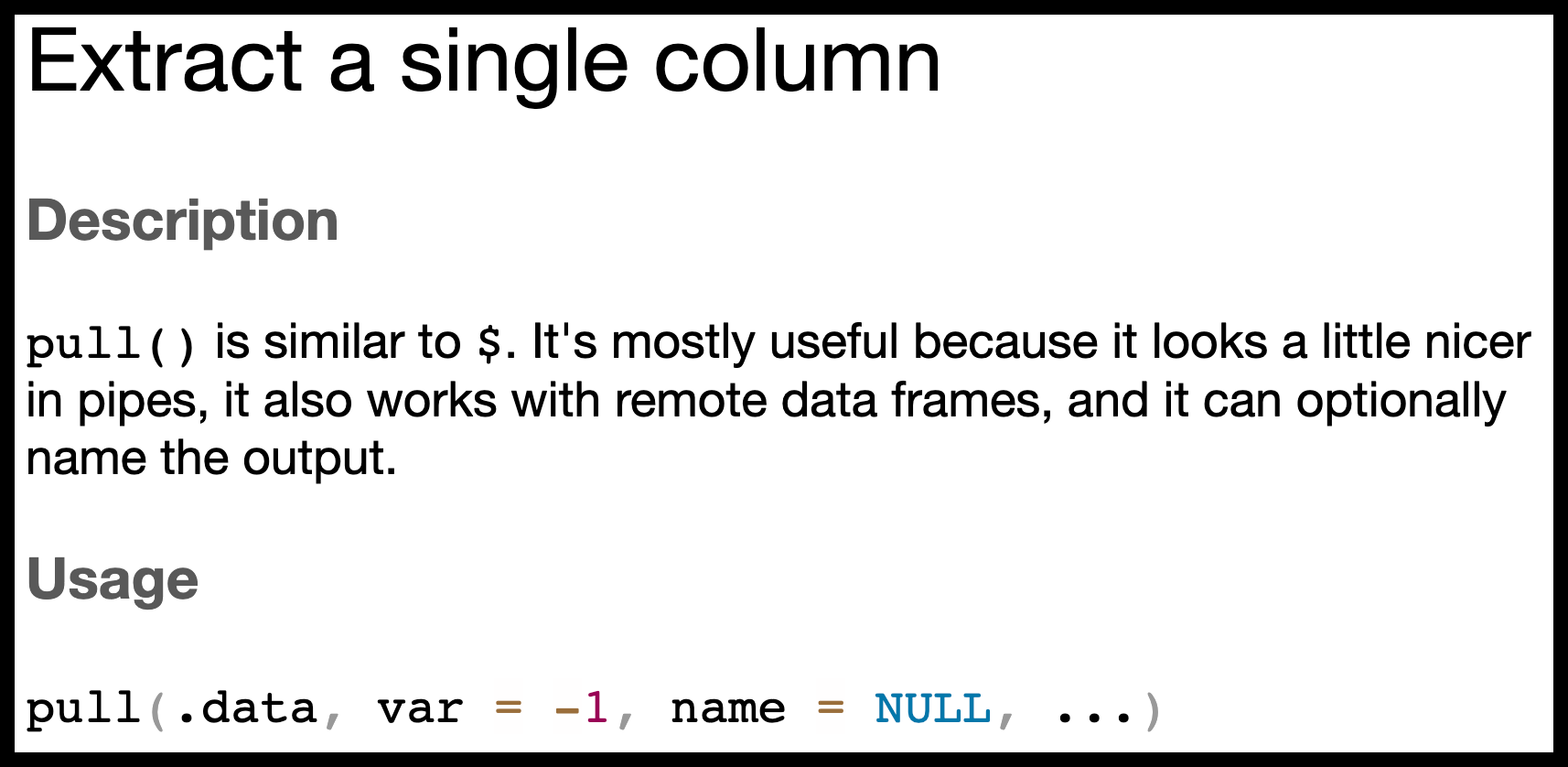
pull() function.
pull() extracts a single column from a data frame and returns it as a vector.
For example, the following code extracts the eye colors of the movie characters and prints the first six values using the head() function:
The Usage section in Figure 4.12 reveals that there are three arguments that can be passed to pull(), named .data, var, and name. The ellipsis ... indicates that additional arguments can be passed, but they are not required.
The second and third argument names (var and name) are each followed by an equals sign (=), whereas there is no equals sign after the first argument (.data). This absence of an equals sign implies that .data does not have a default value, whereas var has a default value of -1 and name has the default value NULL, which is a special value in R, commonly used to indicate the absence of an object.
Arguments with default values are listed in the Usage section in the form arg_name = default.
When invoking a function, it is possible to specify the name of each argument followed by an equals sign (=) and the corresponding value. The following code chunk demonstrates this usage. Please note that, in the third item in the argument list (i.e., name = name), name on the left side of the equals sign stands for the argument name. In contrast, name on the right side stands for the value of the argument, which refers to the column header in starwars that also happens to be called name. By changing the name argument from the value NULL to name, the names of the characters are printed above the eye color:
Use the pattern arg_name = value in a function call to match an argument by name.
Luke Skywalker          C-3PO          R2-D2    Darth Vader    Leia Organa
        "blue"       "yellow"          "red"       "yellow"        "brown"
     Owen Lars
        "blue"
If you are satisfied with the default value, there is no need to include the corresponding argument in the function call. For instance, the following two variables (p_1 and p_2) are identical although the second call to pull() omits the name argument:
The identical() function returns TRUE if and only if the two arguments are exactly the same.
p_1 <- pull(.data = starwars, var = eye_color, name = NULL)
p_2 <- pull(.data = starwars, var = eye_color)
identical(p_1, p_2)
[1] TRUEHowever, it is necessary to specify a value when an argument does not have a default. Otherwise, R will throw an error, as demonstrated in the following example:
pull(var = eye_color, name = NULL)Error: object 'eye_color' not foundWhen specifying arguments by name (i.e., using an equals sign), their order can be altered. For example, the following two calls to the pull() function are equivalent:
An alternative to argument matching by name is matching by position. In that case, the argument name is omitted. For example, the following two calls to the pull() function are equivalent; the first uses named arguments, whereas the second depends on their positions in the argument list:
When the argument name is omitted in the function call, R matches the argument by position.
p_5 <- pull(.data = starwars, var = eye_color, name = name)
p_6 <- pull(starwars, eye_color, name)
identical(p_5, p_6)
[1] TRUEIn the second line above, R assumes that the arguments are arranged in the same order as specified in the Usage section of the help page (Figure 4.12). That is, .data comes first, var comes second, and name is in third position. This requirement contrasts with named matching, which permits arguments to be supplied in any order.
It is common practice to combine positional matching and matching by name, especially when only certain default values require modification. For example, the following code demonstrates matching .data and var by position and name by name:
Luke Skywalker          C-3PO          R2-D2    Darth Vader    Leia Organa
        "blue"       "yellow"          "red"       "yellow"        "brown"
     Owen Lars
        "blue"
Once an argument is matched by name, the remaining arguments should also be matched by name. Otherwise, the code would be difficult to read.
The tidyverse style guide proposes that “data arguments” (in this example: .data) are matched by position and, hence, their names are omitted. Typically, the lack of a default value is an indicator for a data argument. Conversely, it is recommended to match an argument by name when its default value is overridden. Hence, the stylistically preferred version of the previous function call is as follows:
In the argument list, start with positional matching of arguments without default values. Afterward, match any other required arguments by name.
pull(starwars, var = eye_color, name = name)Data analysis often involves a lengthy sequence of function calls. Consider this toy example, performing the following sequence of steps:
rivers vector, which contains the lengths of 141 major North American rivers in miles.rivers using the sample() function.This sequence can be implemented using the following code:
A disadvantage of this code is that the variables tmp_1, tmp_2, and tmp_3 are required for temporary storage. It is possible to eliminate these variables by creating a long chain of function calls:
Unfortunately, the order of the function calls in the code is counterintuitive. When reading the code in the conventional direction from left to right, the first function that appears is print(), followed by pnorm(), sum(), and finally sample(). However, the actual execution order is the opposite: R first performs sample(), then sum() and pnorm(), and finally print().
Moreover, the preceding function call obfuscates which specific argument is passed to each function. For instance, the argument digits = 5 is passed to print(), but it is placed far from the function name, making it difficult to spot the connection.
To enhance readability, it is recommended to use the pipe operator (|>), which can be read as the word “then.” For instance, the sequence of operations above can be succinctly expressed using the pipe operator as follows:
This code chunk looks less convoluted than the previous version because the sequence of the operations follows the order of execution, and the arguments for each function are immediately placed after the function name.
In chains of function calls, use |> to create pipes for improved readability.
While the pipe operator can improve code readability, it should be used judiciously. For example, the following code chunk contains two equivalent invocations of pnorm(), first as a pipe and then as a regular function call. Considering that only one function call is involved, the second option is arguably easier to read. Incidentally, the following code chunk also demonstrates the use of the comment operator (#) to add comments in R code; everything after the # symbol is ignored by R and not executed. This feature is useful for adding explanations or notes to your code:
Use # to add comments in R code. Everything after the # symbol is ignored by R.
Besides avoiding trivially short pipes, it is advisable to refrain from chaining an excessive number of commands with the pipe operator. When a pipe contains more than ten pipe operators, it is preferable to assign a meaningful name to an intermediate object and split the pipe into two shorter pipes. If these recommendations are followed, the pipe operator can be a valuable tool to enhance the readability of R code.
Avoid pipes with only one appearance of |> as well as excessively long pipes.
By now, you have already used numerous R functions, ranging from c() to pull(). The primary purpose of a function is to encapsulate a sequence of commands so that it can be reused later. While most functions you will require in everyday scenarios are already built into R or part of a publicly available package, you will also encounter specific problems that are more elegantly solved by writing your own functions.
The following sections will explain the syntax you must adhere to when writing your own functions (Section 4.5.2.1) and how to specify return values (Section 4.5.2.2).
Consider the following call to R’s built-in message() function:
message("Hello, world!")Every time you execute this line of code, the same message is displayed:
Suppose that you want to greet specific people by name rather than addressing the whole world. Instead of writing a new line of code for every possible addressee, you can modify the message() command as follows. I will explain shortly how and why it works:
say_hello <- function(name) {
message("Hello, ", name, "!")
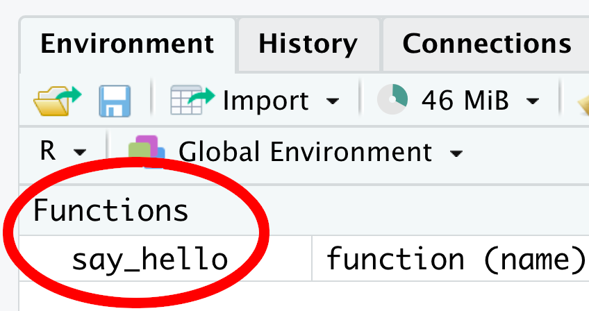
}After executing these lines of code, there will be a function say_hello() in the global environment (Figure 4.13), signalling that R is ready to use this function.
Now, you can enter an argument of your choice inside a pair of parentheses:
say_hello("parallel universe")Hello, parallel universe!Although this is a simple example, it showcases the general syntax of an R function:
The function keyword is required when writing your own function. The argument list must be enclosed in parentheses and can include default default values. The function body is inserted between a pair of braces.
function_name <- function(arg1, arg2, ...) {
  # Body of the function
}
Here are the important features:
Begin with a function name that clearly states the action performed by the function.
After the function name, insert an assignment operator <- followed by the function keyword.
In parentheses, list zero or more arguments.
If required, set a default value for any argument using the syntax arg_name = default. For example, let us choose "world" as default value for name:
say_hello <- function(name = "world") {
  message("Hello, ", name, "!")
}
When running the script and then typing say_hello() in the console without any input, you will greet the whole world:
say_hello()Hello, world!Please note that, even if the parentheses are empty, they should not be omitted. Otherwise, R prints the function code in the console without executing it:
say_hellofunction (name = "world")
{
message("Hello, ", name, "!")
}The ellipsis ... is a special argument that allows the function to accept an arbitrary number of additional arguments. It is useful when you do not know the number of arguments in advance.
Following the argument list, the body of the function is a sequence of instructions whose outputs might depend on the arguments. The body should be enclosed in braces: {}.
Often, the purpose of a function is to return a value. For instance, the next function adds 1 to the x argument and returns the incremented value:
increment <- function(x) {
  return(x + 1)
}
When a value is returned, it can be assigned to a variable (e.g., y) and used later in the Quarto Markdown file:
y <- increment(5)
y
[1] 6A function immediately stops after executing return(). For example, when you run the following commands, the message on the third line is not printed in the output because the function terminated earlier:
The return() function passes a value to the caller and exits the function.
If there is no explicit return() in the function body, the return value is equal to the value of the last executed command. For example, the function below automatically returns the incremented value although there is no explicit return():
The return() function is optional. If it is omitted, the value of the last executed command is returned.
increment <- function(x) {
  x + 1
}
The tidyverse style guide recommends using return() only for early returns. Otherwise, the code should rely on R to return the value of the last evaluated command. Consequently, the version of increment() without return() is stylistically preferred.
Although we will not need to write numerous functions in this book, they will sometimes come in handy to reduce code duplication and, thus, improve readability. If you want to write your own function, you can follow the syntax outlined in this section. Here are the most important features to keep in mind:
().arg_name = default.... allows the function to accept an arbitrary number of additional arguments.{}.In data visualization, ranking vector elements can be invaluable. For instance, when you have limited space in a plot for annotating points representing country-level statistics, you may opt to label only the largest countries. To identify them, you can rank the countries by size and select those with the top ranks for labeling.
The dplyr package provides the min_rank() function for ranking. It assigns rank 1 to the smallest value, rank 2 to the next smallest, and so on. In case of ties, the minimum rank is assigned to all tied elements. For example, if two elements are tied for rank 2, both elements receive rank 2, and the next largest element is assigned rank 4. The following code chunk illustrates this behavior:
The min_rank() function ranks the elements of a vector in ascending order, assigning the rank 1 to the smallest element.
By default, min_rank() assigns 1 to the smallest value. To give rank 1 to the largest value instead, wrap your vector in desc() before ranking, for example:
The desc() function reverses the rank order so that the largest value receives a rank of 1.
A common data-analysis task in R is creating a new vector from an existing one by applying element-wise conditions. The dplyr package provides two convenient functions for this purpose: if_else() (Section 4.7.1) and case_match() (Section 4.7.2).
if_else() for Two-Way Conditional SelectionTo illustrate if_else() in action, consider this simple example. Given a character vector of days (“Monday”, “Tuesday”, …, “Sunday”) we want to create a new vector that assigns “Weekend” to “Saturday” and “Sunday”, whereas all other days are designated as "Weekday".
The if_else() function can solve this problem. It requires at least three arguments:
TRUE if the corresponding element is equal to "Saturday" or "Sunday".TRUE.FALSE:if_else() expects three arguments: a logical test vector, a value to return when the test is TRUE, and a value to return when it is FALSE.
case_match() for Multi-Way Conditional SelectionUnlike if_else(), which supports only two outcomes, case_match() allows specifying multiple return values. For example, you could map "Monday" through "Friday" to "Weekday", leave "Saturday" and "Sunday" unchanged, and assign "Unknown" to any input that isn’t a valid day name.
The case_match() function can return more than two possible values in the output.
The case_match() function handles this situation. As demonstrated in the example below, the arguments use so-called formula syntax—each match pattern appears before a tilde (~), followed by the value to return when that pattern is met—and the .default argument specifies the fallback value if no cases match:
days <- c("Wednesday", "Saturday", "Thursday", "Sunday", NA, "foo")
case_match(
  days,
  "Saturday" ~ "Saturday",
  "Sunday" ~ "Sunday",
  c("Monday", "Tuesday", "Wednesday", "Thursday", "Friday") ~ "Weekday",
  .default = "Unknown"
)
[1] "Weekday" "Saturday" "Weekday" "Sunday" "Unknown" "Unknown" The dplyr functions if_else() and case_match() generate new vectors based on conditions applied to existing logical vectors. Their syntax is:
if_else(condition, true, false), where true specifies the values to return when the condition is TRUE. Otherwise, the value in false is returned.case_match(x, case_1 ~ val_1, case_2 ~ val_2, ..., .default = default_val), where case_i triggers val_i in the output. The .default argument specifies the fallback value if no cases match.Many data sets of interest have a rectangular, spreadsheet-like format. For example, consider the data in Table 4.3, showing the distribution of votes for Bill de Blasio, Nicole Malliotakis, and other candidates in the 2017 New York City mayoral election, broken down by borough. To represent such data in R, data frames are used, which are objects with the following properties:
A data frame is a rectangular data structure where rows correspond to observations and columns to variables. Each column is a vector, and columns can belong to different classes.
| Borough | de Blasio | Malliotakis | Other |
|---|---|---|---|
| Bronx | 117,712 | 23,715 | 3,138 |
| Brooklyn | 254,755 | 74,343 | 10,602 |
| Manhattan | 190,312 | 53,853 | 10,186 |
| Queens | 171,867 | 94,911 | 8,974 |
| Staten Island | 25,466 | 70,125 | 2,747 |
Tibbles form a modern subclass of data frames, as defined in the tibble package, which is part of the tidyverse. Because tibbles are equipped with improved methods for consistent and readable output, they are preferable to generic data frames whenever feasible. Although all data frames discussed in this section will be tibbles, the presented methods apply to data frames in general. Should it be crucial for a data frame to be classified as a tibble, the as_tibble() function can be used for conversion.
Tibbles form a subclass of data frames providing more readable output than generic data frames.
In the rest of this section, you’ll learn how to create data frames from scratch (Section 4.8.1) and how to view their contents (Section 4.8.2).
Tibbles can be created using the tibble() function from the tibble package. The arguments should consist of vectors of equal length, with each vector representing one column in the data frame. Column names can be specified via the argument names. While it is technically possible to include spaces and special characters in column names, it is advisable to stick to letters, numbers, and underscores. Adopting this convention, the code below creates the data frame ny_mayor, containing the data in Table 4.3:
Use tibble() to create a tibble from its constituent vectors.
library(tidyverse)
ny_mayor <- tibble(
  borough = c("Bronx", "Brooklyn", "Manhattan", "Queens", "Staten Island"),
  de_blasio = c(117712, 254755, 190312, 171867, 25466),
  malliotakis = c(23715, 74343, 53853, 94911, 70125),
  other = c(3138, 10602, 10186, 8974, 2747)
)
ny_mayor
# A tibble: 5 × 4
borough de_blasio malliotakis other
<chr> <dbl> <dbl> <dbl>
1 Bronx 117712 23715 3138
2 Brooklyn 254755 74343 10602
3 Manhattan 190312 53853 10186
4 Queens 171867 94911 8974
5 Staten Island 25466 70125 2747Tibbles belong to the data.frame class as well as the tbl_df and tbl subclasses:
class(ny_mayor)[1] "tbl_df" "tbl" "data.frame"The class memberships of a data frame can be confirmed using the is.data.frame() function:
is.data.frame(ny_mayor)[1] TRUEA straightforward method for viewing the content of a data frame is to enter the object name in the console. For data frames with numerous rows or columns, only a subset of the data is displayed. For instance, consider the starwars data frame you encountered in Section 4.4.2:
starwars# A tibble: 87 × 14
name height mass hair_color skin_color eye_color birth_year sex gender
<chr> <int> <dbl> <chr> <chr> <chr> <dbl> <chr> <chr>
1 Luke Sk… 172 77 blond fair blue 19 male mascu…
2 C-3PO 167 75 <NA> gold yellow 112 none mascu…
3 R2-D2 96 32 <NA> white, bl… red 33 none mascu…
4 Darth V… 202 136 none white yellow 41.9 male mascu…
5 Leia Or… 150 49 brown light brown 19 fema… femin…
6 Owen La… 178 120 brown, gr… light blue 52 male mascu…
7 Beru Wh… 165 75 brown light blue 47 fema… femin…
8 R5-D4 97 32 <NA> white, red red NA none mascu…
9 Biggs D… 183 84 black light brown 24 male mascu…
10 Obi-Wan… 182 77 auburn, w… fair blue-gray 57 male mascu…
# ℹ 77 more rows
# ℹ 5 more variables: homeworld <chr>, species <chr>, films <list>,
# vehicles <list>, starships <list>To determine the number of rows and columns in a data frame, you can use the nrow() and ncol() functions:
To retrieve the first few rows of a data frame, the head() function can be used:
head(starwars)# A tibble: 6 × 14
name height mass hair_color skin_color eye_color birth_year sex gender
<chr> <int> <dbl> <chr> <chr> <chr> <dbl> <chr> <chr>
1 Luke Sky… 172 77 blond fair blue 19 male mascu…
2 C-3PO 167 75 <NA> gold yellow 112 none mascu…
3 R2-D2 96 32 <NA> white, bl… red 33 none mascu…
4 Darth Va… 202 136 none white yellow 41.9 male mascu…
5 Leia Org… 150 49 brown light brown 19 fema… femin…
6 Owen Lars 178 120 brown, gr… light blue 52 male mascu…
# ℹ 5 more variables: homeworld <chr>, species <chr>, films <list>,
# vehicles <list>, starships <list>Another option is to use the glimpse() function from the dplyr package, which provides a compact overview of the data frame’s structure. The output shows the row and column counts, column names and classes, and the first few values:
Use glimpse() for a concise display of a data frame’s structure.
glimpse(starwars)Rows: 87
Columns: 14
$ name <chr> "Luke Skywalker", "C-3PO", "R2-D2", "Darth Vader", "Leia Or…
$ height <int> 172, 167, 96, 202, 150, 178, 165, 97, 183, 182, 188, 180, 2…
$ mass <dbl> 77.0, 75.0, 32.0, 136.0, 49.0, 120.0, 75.0, 32.0, 84.0, 77.…
$ hair_color <chr> "blond", NA, NA, "none", "brown", "brown, grey", "brown", N…
$ skin_color <chr> "fair", "gold", "white, blue", "white", "light", "light", "…
$ eye_color <chr> "blue", "yellow", "red", "yellow", "brown", "blue", "blue",…
$ birth_year <dbl> 19.0, 112.0, 33.0, 41.9, 19.0, 52.0, 47.0, NA, 24.0, 57.0, …
$ sex <chr> "male", "none", "none", "male", "female", "male", "female",…
$ gender <chr> "masculine", "masculine", "masculine", "masculine", "femini…
$ homeworld <chr> "Tatooine", "Tatooine", "Naboo", "Tatooine", "Alderaan", "T…
$ species <chr> "Human", "Droid", "Droid", "Human", "Human", "Human", "Huma…
$ films <list> <"A New Hope", "The Empire Strikes Back", "Return of the J…
$ vehicles <list> <"Snowspeeder", "Imperial Speeder Bike">, <>, <>, <>, "Imp…
$ starships <list> <"X-wing", "Imperial shuttle">, <>, <>, "TIE Advanced x1",…A similar overview can be obtained by clicking on the arrow next to the data frame’s name in the Environment tab of RStudio’s top right pane, as shown in Figure 4.14:
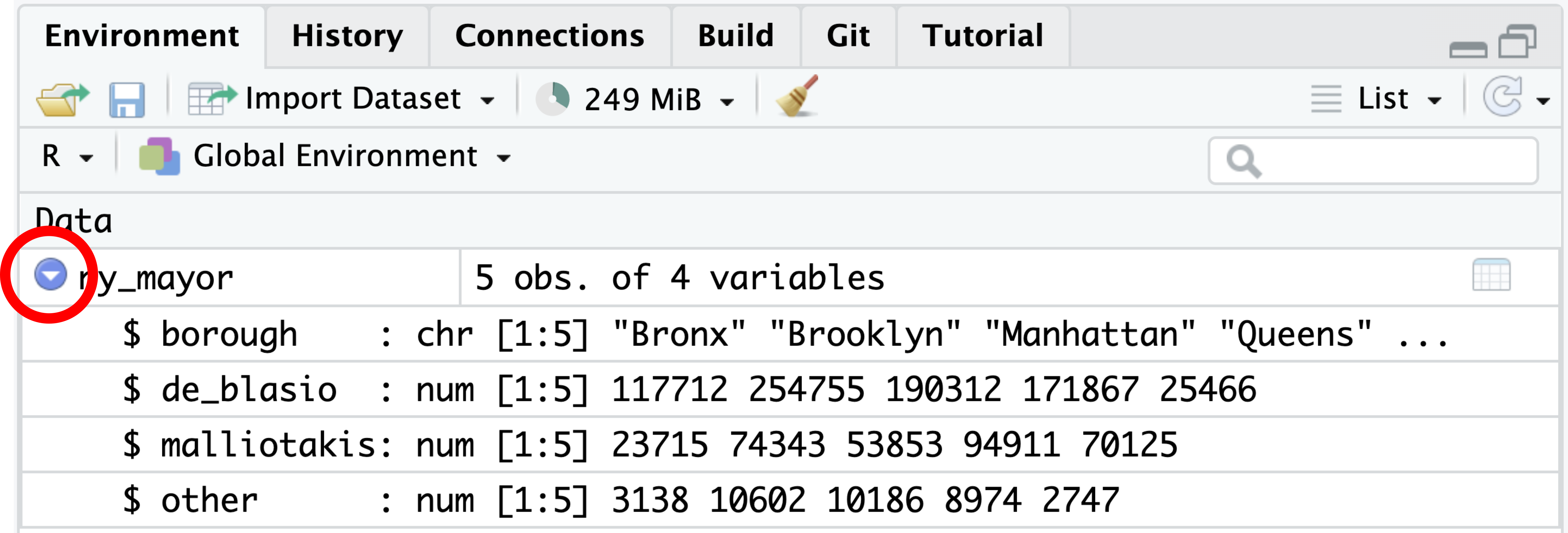
ny_mayor. Clicking the arrow (highlighted in red) expands the list to reveal each column’s name, data type, and initial values. Clicking the variable name opens the spreadsheet view shown in Figure 4.15.
For a more comprehensive inspection of the data, you can use the View() function, which opens a spreadsheet in RStudio’s top left pane, as depicted in Figure 4.15:
Use View() to open a spreadsheet view of a data frame.
View(starwars)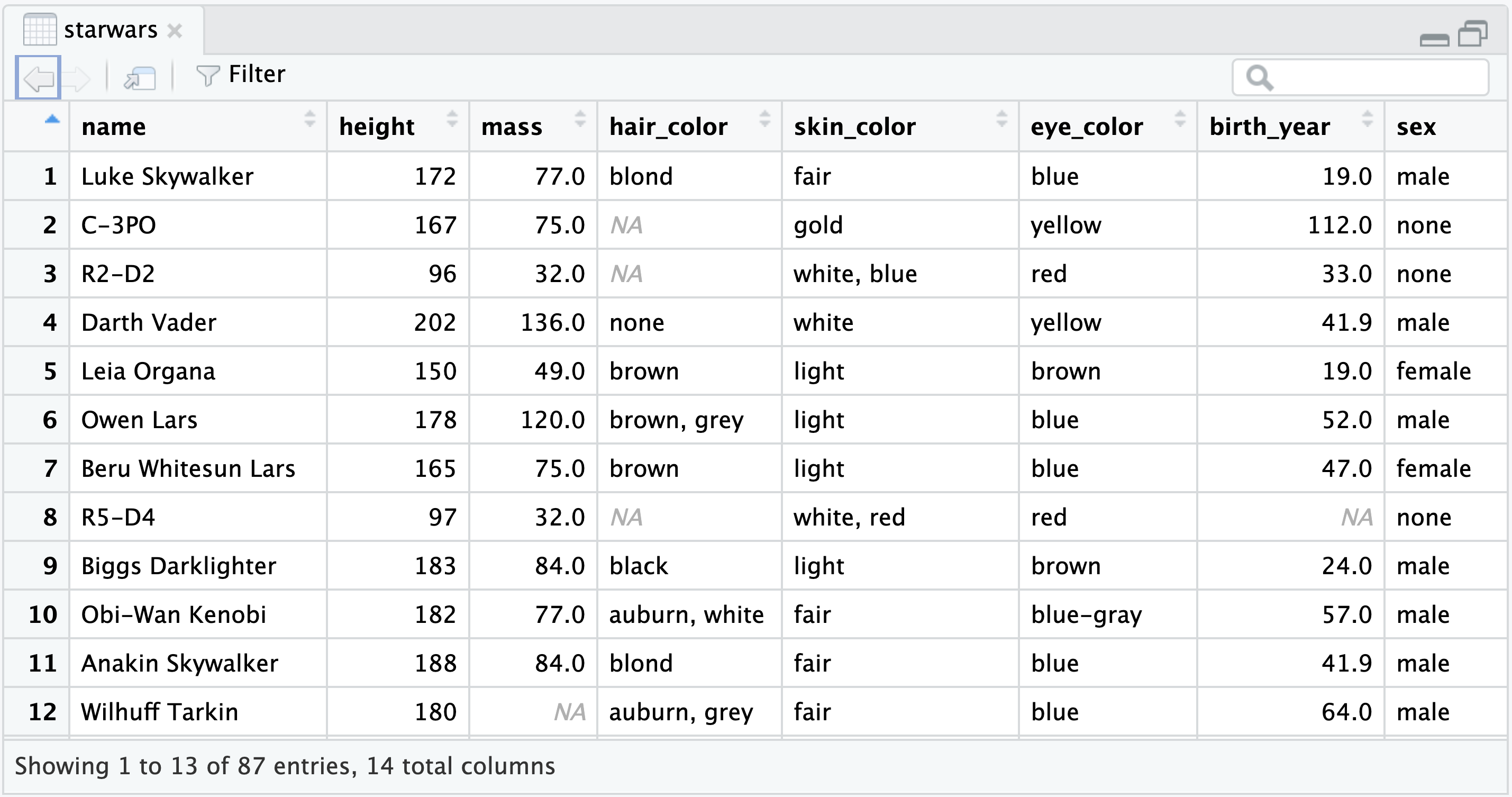
starwars data frame.
Alternatively, you can click the line containing the data frame’s variable name in the Environment tab to open the spreadsheet view.
$
When working with a data frame, you often need to extract a single column as a vector. As demonstrated in Section Section 4.5.1, you can use pull() for this purpose. Alternatively, the $ operator achieves the same result. For example, the code below extracts the borough column from the ny_mayor data frame:
The $ operator extracts a column vector from a data frame.
ny_mayor$borough[1] "Bronx" "Brooklyn" "Manhattan" "Queens"
[5] "Staten Island"Although pull() integrates seamlessly into pipelines, the $ operator is more convenient for interactive exploration at the console.
In Section 4.8, you manually entered the data for the 2017 New York City mayoral election using the tibble() function. While this approach is feasible for small data sets, it is usually impractical to hard-code larger amounts of data into a code chunk. Instead, such data sets are often stored in spreadsheet files. In this section, you will learn how to import spreadsheet data from two common file types: Comma-separated values (CSV; Section 4.9.1) and Excel Spreadsheets (XLSX or XLS; Section 4.9.2).
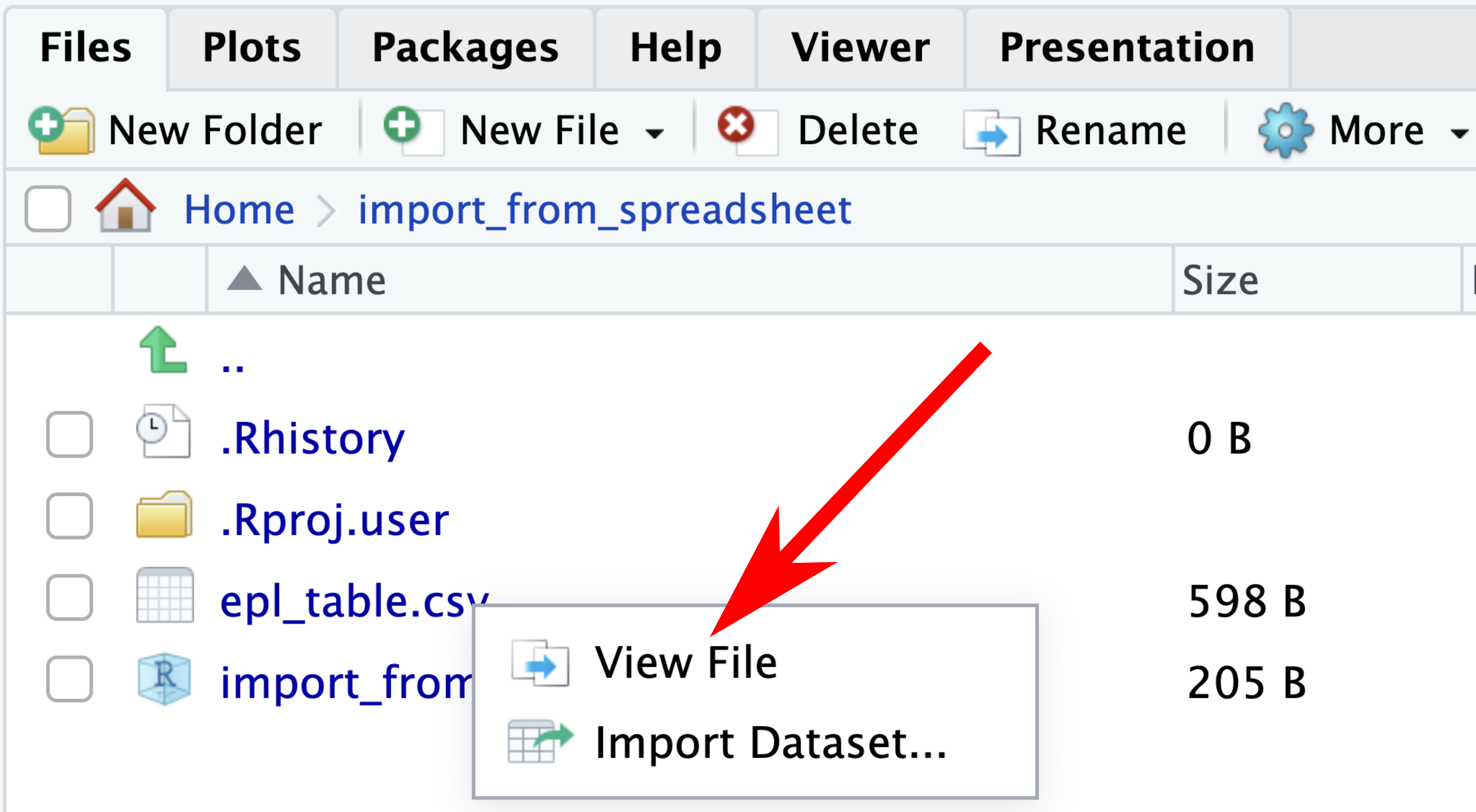
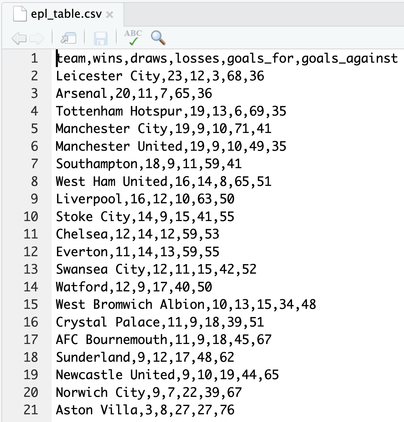
We will work with a sample data set available from the book website, containing the final English Premier League football table for the 2015–16 season. Please move this file to your project directory and click its name in the Files tab, located in RStudio’s bottom right pane. From the context menu, click “View File” (Figure 4.16) which opens a plain-text view in the top left pane (Figure 4.17).
Inspecting the content of the file reveals typical features of the CSV file format:
CSV files can be imported into R by either using the RStudio GUI or running R commands at the console or in a QMD file. When importing the file for the first time, it is often quicker to resort to the GUI, which automatically generates the necessary R commands that can be copied and pasted into a QMD file for future use. To launch the GUI, simply click the CSV file name in the Files tab and, then, on “Import Dataset…”
If you are unfamiliar with a data set, use the “Import Text Data” GUI to import it.
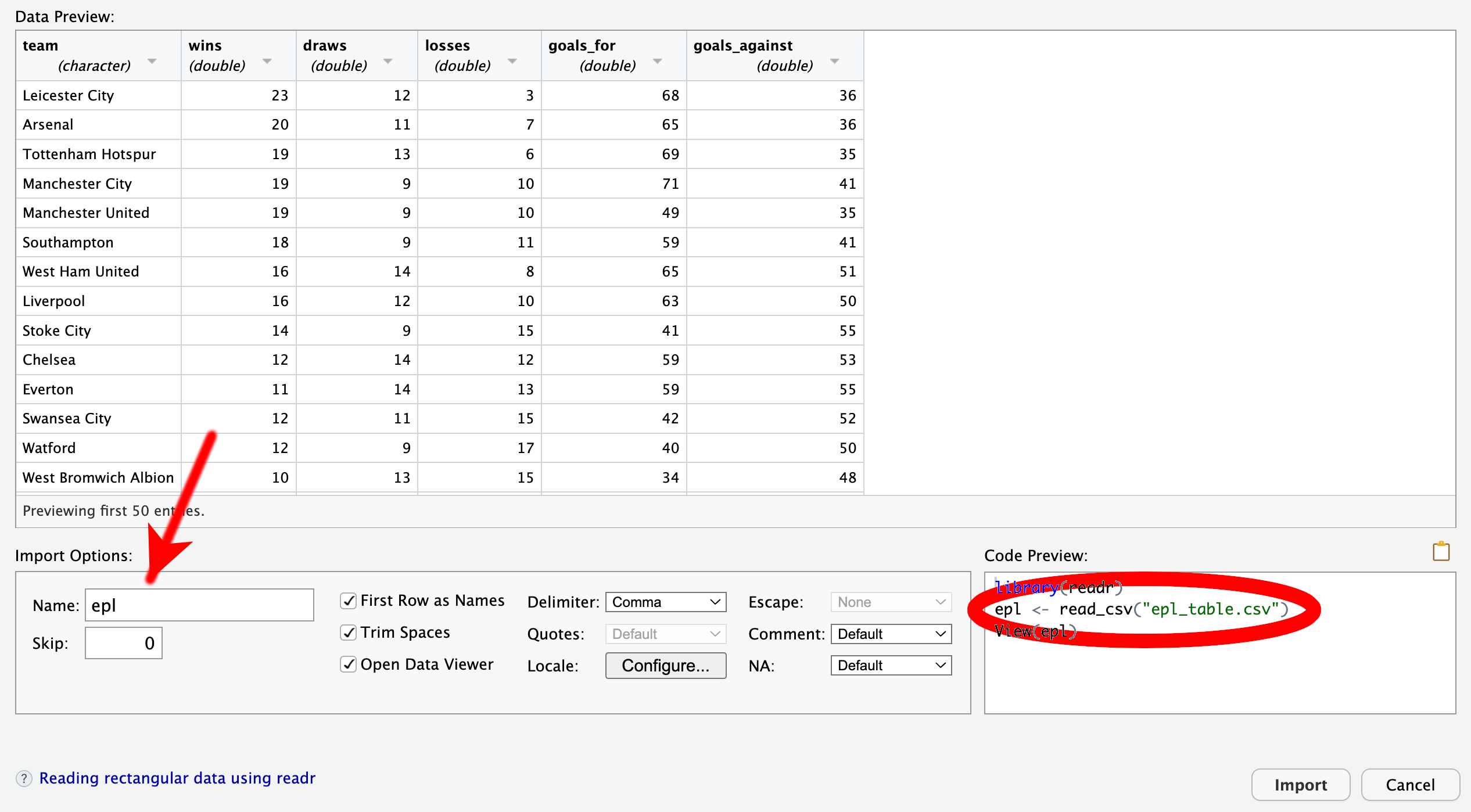
The initial preview of the data in the GUI (Figure 4.18) displays R’s attempt to parse the data by row and column. Sometimes, certain options in the bottom of the GUI require adjustments. For example, CSV files authored in some European countries may require changing the delimiter from “Comma” to “Semicolon.” However, in the current case, the data are correctly split into spreadsheet cells. In principle, you could proceed by clicking the “Import” button now, but I recommend that you take a closer look at the “Code Preview” in the bottom right of the dialog window.
The code preview consists of three lines:
library(readr), loads the readr package, which contains utility functions for importing tabular data. It is part of the tidyverse. Thus, if the QMD file has already loaded the entire tidyverse suite using library(tidyverse), then there is no longer any need to call library(readr). In that case, this line of code should be removed for conciseness.read_csv(), one of the functions in readr. By default, the imported data would be assigned to a tibble named epl_table. If you prefer another name, such as the more concise epl, you can edit the “Name” field of the GUI, highlighted in Figure 4.18.View(), which opens a spreadsheet view of the data frame. While this function can be helpful for exploring the data interactively, it does not serve any purpose in a QMD file. Therefore, I recommend removing this line. If you want to provide the reader with an overview of the data, it is better to use functions like head() or glimpse().Use read_csv() to import CSV files.
Calls to read_csv() automatically generate control output, displaying the inferred data type of each column. Because this information is typically not of interest to readers of the rendered document, I recommend turning off the control output using the execution option message: false, as explained in Section 3.4.4.3.
In summary, a code chunk for importing data from a CSV file might look similar to the following example:
```{r}
#| label: read-csv
#| message: false

epl <- read_csv("epl_table.csv")
```While a CSV file is often the preferred option for storing spreadsheet data because of its simplicity, many data sets are only available in Excel format. A sample file, saved in Excel’s XLSX format, can be found on the book website. Please transfer this file to your project directory. To import the data, click the XLSX file name in the Files tab and choose “Import Dataset…” from the context menu to launch the “Import Excel Data” GUI (Figure 4.19).
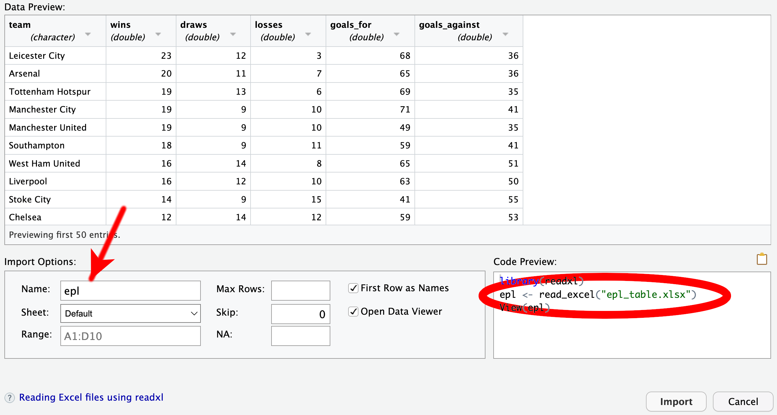
The options at the bottom of this GUI differ slightly from those in the “Import Text Data” GUI that you encountered when importing a CSV file in Section 4.9.1. For instance, there is now a dropdown menu named “Sheet” because Excel files can consist of multiple sheets, unlike CSV files. The code preview also exhibits minor differences. First, the package required for importing Excel files is readxl instead of readr. Unlike readr, readxl is not part of the tidyverse; thus, the library(readxl) needs to be invoked before importing Excel files, even if library(tidyverse) has been called. Instead of read_csv(), the second line of the code preview now calls the function read_excel(). You can find more information about read_excel() and other functions in the readxl package by running help(package = "readxl"). The documentation explains that read_excel() needs to guess whether the file is in XLSX or XLS format. If the user already knows the format, it is preferable to use read_xlsx() or read_xls() instead. Thus, a code chunk for importing an XLSX file might follow this pattern:
Use read_xlsx() to import XLSX files and read_xls() for XLS files.
```{r}
#| label: read-xlsx

library(readxl) # Move this line to the top of the QMD file
epl <- read_xlsx("epl_table.xlsx")
```So far, you have worked with vectors that belonged to the classes numeric, character, and logical. In this section, you will encounter a new class, called factor, which is R’s data structure for representing categorical data. Factors are more complex than the simple vectors you have dealt with until now. However, factors offer more effective solutions for tasks involving categorical data.
Prompted by an inspection of a built-in factor in Section 4.10.1, the need for factors will be explained in Section 4.10.2. Then, you will discover how to create factors (Section 4.10.3) and operate on the set of possible categories, referred to as “levels” (Section 4.10.4). Afterward, you will learn techniques for tallying levels and sorting them by frequency (Section 4.10.5). Lastly, Section 4.10.6 will discuss the distinction between nominal and ordinal data, with the latter requiring the use of the ordered subclass of factors.
R ships with several built-in data sets about US states, such as the character vector state.name:
state.name [1] "Alabama" "Alaska" "Arizona" "Arkansas"
[5] "California" "Colorado" "Connecticut" "Delaware"
[9] "Florida" "Georgia" "Hawaii" "Idaho"
[13] "Illinois" "Indiana" "Iowa" "Kansas"
[17] "Kentucky" "Louisiana" "Maine" "Maryland"
[21] "Massachusetts" "Michigan" "Minnesota" "Mississippi"
[25] "Missouri" "Montana" "Nebraska" "Nevada"
[29] "New Hampshire" "New Jersey" "New Mexico" "New York"
[33] "North Carolina" "North Dakota" "Ohio" "Oklahoma"
[37] "Oregon" "Pennsylvania" "Rhode Island" "South Carolina"
[41] "South Dakota" "Tennessee" "Texas" "Utah"
[45] "Vermont" "Virginia" "Washington" "West Virginia"
[49] "Wisconsin" "Wyoming" class(state.name)[1] "character"Another data set, state.region, denotes the region (Northeast, South, North Central, or West) to which each state belongs:
state.region [1] South West West South West
[6] West Northeast South South South
[11] West West North Central North Central North Central
[16] North Central South South Northeast South
[21] Northeast North Central North Central South North Central
[26] West North Central West Northeast Northeast
[31] West Northeast South North Central North Central
[36] South West Northeast Northeast South
[41] North Central South South West Northeast
[46] South West South North Central West
Levels: Northeast South North Central WestAt first glance, state.region might appear to be a character vector; however, comparing its output to that of state.name reveals two important distinctions. First, the character strings in the output of state.region are not enclosed in quotation marks. Second, an additional line appears at the end of the output of state.region, starting with the word “Levels.”
This unfamiliar output format arises because state.region is a factor, not a character vector, as the class() function reveals:
class(state.region)[1] "factor"To confirm that an R object is a factor, the is.factor() function can be used:
is.factor(state.region)[1] TRUEWhat is the purpose of the factor class? To answer this question, let us briefly consider the classifications of data types in statistics.
Statistical data can be broadly categorized into three classes:
Unique values associated with individual observations. Examples include:
Numbers that allow meaningful arithmetic operations, such as addition or multiplication. Examples include:
state.area vector)Classifications that split observations into a small number of groups or categories, for example:
Statistical data encompass identifiers, quantitative data, and categorical data.
Frequently, character strings are used for labeling groups of categorical data, but numbers can also be used. For example, an opinion poll might represent “I agree” by +1, “No opinion” by 0, and “I disagree” by -1. However, these numbers lack any arithmetic connotation. It would not make sense, for instance, to regard the sum of “I agree” and “I disagree” as equal to “No opinion.”
Although categories can be represented as words or numbers, generic numeric or character vectors differ semantically from categorical variables. The essence of categorical data lies in the meaning attributed to each category rather than the name or number with which it is labelled. For this reason, it is desirable to have a data structure that allows, for example, renaming a category without changing the semantics of the represented data. Factors in R are tailored to fulfill this need and handle various other tasks specific to categorical data.
Factors form a data structure designed for handling categorical data.
Consider a globally operating coffee-house chain named StellaDollari, financed by discreet state investors based in countries with growth potential in their freedom-of-press ranking. StellaDollari offers beverages in the sizes “Modesto,” “Regolare,” “Pomposo,” and “Colossale.” Outperforming its legal obligations, StellaDollari clandestinely collects personally identifiable information about its customers, including the drink sizes they order. These sizes can be regarded as categorical data, and, thus, factors are a suitable class for storing this information. Suppose that the first four customers ordered the sizes Pomposo, Colossale, Pomposo again, and Regolare. You can create a factor consisting of these data using the factor() function:
Use the factor() function to create a factor.
[1] Pomposo   Colossale Pomposo   Regolare
Levels: Colossale Pomposo Regolare
In R terminology, the levels on the last line of output represent the labels of the categories, listed in alphabetical order by default. In the example above, there are three levels: Colossale, Pomposo, and Regolare.
But wait! Weren’t there four categories? What happened to the Modesto category? R was not aware of its existence because it did not appear in the input. To inform R about all possible category labels, you need to pass the levels argument to factor():
Use the levels argument to specify the names of all possible categories.
sizes <- factor(
  c("Pomposo", "Colossale", "Pomposo", "Regolare"),
  levels = c("Modesto", "Regolare", "Pomposo", "Colossale")
)
sizes
[1] Pomposo Colossale Pomposo Regolare
Levels: Modesto Regolare Pomposo ColossaleIn the final line of output, the levels appear in the order specified in the levels argument, now including the previously missing Modesto category.
If the levels argument fails to specify all levels appearing in the first argument, the output will contain NA:
The levels() function retrieves the levels in a factor:
Use levels() to retrieve the levels.
levels(sizes)[1] "Modesto" "Regolare" "Pomposo" "Colossale"Suppose that you wish to abbreviate the levels as m, r, p, and c. You can change the levels with fct_recode() from the forcats package, which contains many useful functions for working with factors:
Use fct_recode() to change the labels of factor levels.
library(forcats)
fct_recode(
  sizes,
  m = "Modesto",
  r = "Regolare",
  p = "Pomposo",
  c = "Colossale"
)
[1] p c p r
Levels: m r p cIf the input contains the same category under different names, you can merge the levels using fct_collapse() from the forcats package:
Use fct_collapse() to merge categories.
[1] "Big" "Pomposo" "r" # Combine "Pomposo" and "Big" into the new category "p"
fct_collapse(proportions, p = c("Pomposo", "Big"))[1] p p r
Levels: p rFactors containing many levels can be cumbersome to work with. For effective communication it can be beneficial to gather several levels that are not of individual relevance into a single category, often termed “Other.” The fct_other() function from the forcats package can be used for this purpose:
Use fct_other() to merge levels into “Other.”
It is often useful to count the number of occurrences of each category in a data set. Consider the example of the gss_cat data frame from the forcats package, which contains a sample of 21,483 responses in the General Social Survey. This biannual survey, conducted by the National Opinion Research Center at the University of Chicago, collects demographic information from representative respondents in the US population, along with their opinions, attitudes, and behaviors. Here is a compact display of the content in gss_cat:
glimpse(gss_cat)Rows: 21,483
Columns: 9
$ year <int> 2000, 2000, 2000, 2000, 2000, 2000, 2000, 2000, 2000, 2000, 20…
$ marital <fct> Never married, Divorced, Widowed, Never married, Divorced, Mar…
$ age <int> 26, 48, 67, 39, 25, 25, 36, 44, 44, 47, 53, 52, 52, 51, 52, 40…
$ race <fct> White, White, White, White, White, White, White, White, White,…
$ rincome <fct> $8000 to 9999, $8000 to 9999, Not applicable, Not applicable, …
$ partyid <fct> "Ind,near rep", "Not str republican", "Independent", "Ind,near…
$ relig <fct> Protestant, Protestant, Protestant, Orthodox-christian, None, …
$ denom <fct> "Southern baptist", "Baptist-dk which", "No denomination", "No…
$ tvhours <int> 12, NA, 2, 4, 1, NA, 3, NA, 0, 3, 2, NA, 1, NA, 1, 7, NA, 3, 3…The relig column in gss_cat reports the religions of the participants using the following levels:
 [1] "No answer"               "Don't know"
 [3] "Inter-nondenominational" "Native american"
 [5] "Christian"               "Orthodox-christian"
 [7] "Moslem/islam"            "Other eastern"
 [9] "Hinduism"                "Buddhism"
[11] "Other"                   "None"
[13] "Jewish"                  "Catholic"
[15] "Protestant"              "Not applicable"
To determine the frequency of each response, the fct_count() function can be invoked:
Use fct_count() to count the frequency of each level in a factor.
fct_count(relig)# A tibble: 16 × 2
f n
<fct> <int>
1 No answer 93
2 Don't know 15
3 Inter-nondenominational 109
4 Native american 23
5 Christian 689
6 Orthodox-christian 95
7 Moslem/islam 104
8 Other eastern 32
9 Hinduism 71
10 Buddhism 147
11 Other 224
12 None 3523
13 Jewish 388
14 Catholic 5124
15 Protestant 10846
16 Not applicable 0The output lines are in the same order as the levels. However, it would be more insightful if the categories were sorted such that the most frequent response appears at the top. This task can be achieved in two stages. First, the levels can be reordered in descending order of frequency using fct_infreq() from the forcats package:
Use fct_infreq() to order the levels by frequency.
relig_descending <- fct_infreq(relig)
levels(relig_descending)
[1] "Protestant" "Catholic"
[3] "None" "Christian"
[5] "Jewish" "Other"
[7] "Buddhism" "Inter-nondenominational"
[9] "Moslem/islam" "Orthodox-christian"
[11] "No answer" "Hinduism"
[13] "Other eastern" "Native american"
[15] "Don't know" "Not applicable" Second, fct_count() is applied to the factor with the reordered levels:
fct_count(relig_descending)# A tibble: 16 × 2
f n
<fct> <int>
1 Protestant 10846
2 Catholic 5124
3 None 3523
4 Christian 689
5 Jewish 388
6 Other 224
7 Buddhism 147
8 Inter-nondenominational 109
9 Moslem/islam 104
10 Orthodox-christian 95
11 No answer 93
12 Hinduism 71
13 Other eastern 32
14 Native american 23
15 Don't know 15
16 Not applicable 0The output reveals that the most frequent response is “Protestant.”
Categorical data can be classified into two distinct types: nominal and ordinal. Nominal data consist of categories that have no inherent order, whereas categories of ordinal data can be meaningfully sorted. Examples of nominal data are nationality, religion, and AC power plug type, whereas examples of ordinal data include opinions on a Likert scale (spanning from “Disagree” over “Neutral” to “Agree”), military ranks, or StellaDollari drink sizes (ranging from “Modesto” over “Regolare” and “Pomposo” to “Colossale”).
Ordinal data can be compared meaningfully using inequality operators. For example, it is reasonable to regard "Regolare" < "Pomposo" as TRUE. However, when using R’s default factors, any comparison of levels with the ordered inequality operators (<, >, <=, and >=) produces NA:
sizes[1] Pomposo Colossale Pomposo Regolare
Levels: Modesto Regolare Pomposo Colossalesizes > "Pomposo"Warning in Ops.factor(sizes, "Pomposo"): '>' not meaningful for factors[1] NA NA NA NAThe warning message implies that factors are, by default, assumed to represent nominal data. For ordinal data, a more specialized R data structure is required, known as an ordered factor. To create an ordered factor, the argument ordered = TRUE must be be passed to the factor() function:
Ordinal data should be stored in ordered factors. Invoke factors() with ordered = TRUE to create an ordered factor.
The ordered = TRUE argument adds the result to the ordered class:
Ordered factors belong to the ordered subclass of the factor class.
class(sizes_ord)[1] "ordered" "factor" Membership in the ordered class can be confirmed using the is.ordered() function:
is.ordered(sizes_ord)[1] TRUEUnlike for conventional factors, ordered factors allow comparisons with ordered inequality operators, for example:
Ordered factors support comparisons using <, >, <=, and >=.
sizes_ord > "Pomposo"[1] FALSE TRUE FALSE FALSEBecause ordered factors inherit the methods of conventional factors, all the functions in the previous sections, such as fct_recode() and fct_count(), can be applied to them, and the results will themselves be ordered factors. However, the ordering of the levels might not be meaningful if levels are merged or shuffled. In that case, it might be sensible to convert the input to an unordered factor using factor() with the ordered = FALSE argument.
When working with categorical data, it is advisable to represent them as factors, for which R has native support:
factor() function.levels() function retrieves the levels in a factor.ordered subclass represents ordinal data.The forcats package adds many practical utility functions. The official forcats cheatsheet provides a concise overview of the available options. You may want to consult this resource while coding.
Throughout this chapter, you have acquired essential R programming skills. You have become familiar with fundamental data structures (such as vectors, data frames, and factors) as well as functions. You have also learned how to seek help, integrate third-party packages into your code, and import data from files. We conclude with a glossary in Table 4.4, summarizing the most important terms and concepts introduced in this chapter.
| Term | Definition |
|---|---|
| Argument | An input to a function, specified by position or by name. Some arguments may have default values. |
Assignment operator (<-) |
The symbol used to assign a value to a variable (e.g., x <- 42). |
| Conditional element selection | A method to select elements of a vector from a list of alternatives. The if_else() and case_match() functions in the dplyr package provide this functionality. |
| Data frame | A rectangular tabular object where rows are observations and columns represent variables. Each column is a vector, which can be retrieved using dplyr::pull() or $. |
Dollar sign operator ($) |
An operator to access a specific column of a data frame (e.g., dfr$col_name). |
Double-colon operator (::) |
An operator to access a specific object from a package without attaching the entire package. Usage: dplyr::pull(). |
| Factor | A data structure for categorical data. Observations are classified into categories that are stored in the levels attribute. |
| Function | An R object that performs a task dependent on input arguments. Functions are invoked by their name followed by parentheses (e.g., sum(1:10)). |
Help operator (?) |
Documentation shortcut. It opens R’s built-in help page of a known object. For example, ?seq retrieves the help page of the seq() function. |
| Logical vector | A vector whose elements can only be TRUE, FALSE, or NA. |
Missing value (NA) |
A special placeholder indicating “Not available”. |
| Ordered factor | A factor with a defined order among its levels, enabling comparisons like < and >. |
| Package | A bundle of R functions, data, and documentation that extends R’s base capabilities. Packages can be loaded with library(). |
| Pipe operator ( |>) |
An operator that passes the output of one expression as first argument to the next expression. |
| Tibble | A data-frame subclass with improved console output. |
| Vector | A R object whose elements all share the same class (e.g., numeric, character, or logical). |
Suppose a student wants to inspect the band_members data set in the dplyr package by executing the following command in the console:
band_membersThe student receives this error message:
Error: object 'band_members' not foundTrying to find the reason for the error, the student finds that RStudio’s Packages tab displays the information shown in figure Figure 4.20.
What action will enable the student to successfully execute the band_members command?
As you will learn in Section 4.2, logical vectors—as well as vectors of any other type—can also contain missing values in the form of NA, which stands for “Not Assigned.”↩︎