13  Visualizing Geospatial Data

Statistical data often relate to geographic locations. The data may contain information about administrative units (e.g., countries or provinces), divide the surface of the earth into categories (e.g., climate zones), or identify specific coordinates (e.g., earthquake epicenters). In this chapter, you will learn how to visualize common types of geospatial data using ggplot2.

Our exploration will center on data represented as “Simple Features,” which are a set of standards established by the Open Geospatial Consortium to describe geospatial objects, such as points, lines, or polygons. Simple Features are widely supported across various software platforms, notably R’s sf package, providing sf objects, which augment the conventional data frame class to manage geospatial data. Section 13.1 will outline the core components of an sf object and the import of geospatial data into sf objects. Subsequently, Section 13.2 will address strategies for handling common challenges when working with geospatial data, such as repairing an invalid topology and simplifying overly detailed geometries. Another critical aspect of geospatial data visualization is the coordinate reference system (CRS). As Section 13.3 will explain, the CRS defines the map projection, establishing a correspondence between the Earth’s nearly spherical surface and a two-dimensional plane, such as a paper map or a digital display.

For data associated with administrative units, the most common map type is the choropleth map, which will be the topic of Section 13.4. Choropleth maps use color to represent the value of an intensive variable, such as population density or an annual percentage change in GDP.

13.1 Simple Features: the sf Class

To create a map using a computer, data must be stored in data structures suitable for geospatial information. In R, the sf class provides a user-friendly geospatial extension of data frames for this purpose. This chapter introduces the sf class and demonstrates how to work with sf objects.

As demonstrated in Section 13.1.1, sf objects encapsulate the geometric information in a special geometry column. This column is essential for plotting maps, as illustrated in Section 13.1.2. Because maps can contain different geometric objects, the sf class can represent points, lines, and polygons, as explained in Section 13.1.3. These objects are typically stored in specialized geospatial file formats, such as GeoJSON or shapefiles. Section 13.1.4 will guide you through the process of importing these files into R.

13.1.1 Geometry Encoded in sf Objects

An example of an sf object is the World data set from the tmap package. The class() function reveals that World, like all sf objects, belongs to both the sf and data.frame classes:

data(World, package = "tmap")
class(World)

[1] "sf"         "data.frame"

Because every sf object is a data frame, you can apply familiar tidyverse functions, such as select(), filter(), and left_join(). For example, the code below demonstrates how to select the iso_a3 and name columns of World:

library(sf)
countries <- select(World, iso_a3, name)
countries

Simple feature collection with 177 features and 2 fields
Attribute-geometry relationships: identity (2)
Geometry type: MULTIPOLYGON
Dimension:     XY
Bounding box:  xmin: -180 ymin: -90 xmax: 180 ymax: 83.645
Geodetic CRS:  WGS 84
First 10 features:
   iso_a3        name                       geometry
1     AFG Afghanistan MULTIPOLYGON (((66.217 37.3...
2     ALB     Albania MULTIPOLYGON (((20.605 41.0...
3     DZA     Algeria MULTIPOLYGON (((-4.923 24.9...
4     AGO      Angola MULTIPOLYGON (((12.322 -6.1...
5     ATA  Antarctica MULTIPOLYGON (((-61.883 -80...
6     ARG   Argentina MULTIPOLYGON (((-68.634 -52...
7     ARM     Armenia MULTIPOLYGON (((46.483 39.4...
8     AUS   Australia MULTIPOLYGON (((147.689 -40...
9     AUT     Austria MULTIPOLYGON (((16.88 48.47...
10    AZE  Azerbaijan MULTIPOLYGON (((46.144 38.7...

At first glance, it may seem surprising that, in addition to the selected iso_a3 and name columns, the output includes a geometry column, even though no column with this name was explicitly selected. The geometry column is a defining feature of every sf object, containing the geospatial context of all observations.¹ Consequently, the output of select() still includes this column so that the returned object remains a valid sf object. To remove this column, the st_drop_geometry() function from the sf package can be used. However, doing so will strip the object of its sf classification. Note that almost all functions in the sf package are prefixed with st_, which stands for “spatial type”:

The sf class is a subclass of data.frame, characterized by the presence of a geometry column.

countries <- st_drop_geometry(countries)
slice_head(countries, n = 5)

  iso_a3        name
1    AFG Afghanistan
2    ALB     Albania
3    DZA     Algeria
4    AGO      Angola
5    ATA  Antarctica

class(countries)

[1] "data.frame"

Henceforth, I will frequently use functions from the sf package, implicitly assuming that it has been loaded using library(sf).

13.1.2 Visualizing sf Objects Using geom_sf()

The ggplot2 package provides the geom_sf() function for visualizing sf objects. For instance, the code below creates a basic map of the World data set:

Use geom_sf() to plot an sf object.

ggplot(World) +
  geom_sf()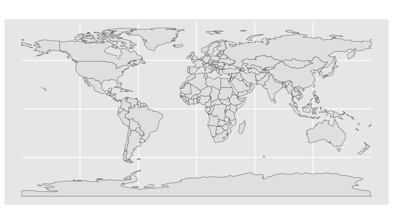

The geom_sf() function can handle a variety of aesthetics. For example, the fill aesthetics fills the inside of the polygons with color:

ggplot(World, aes(fill = continent)) +
  geom_sf()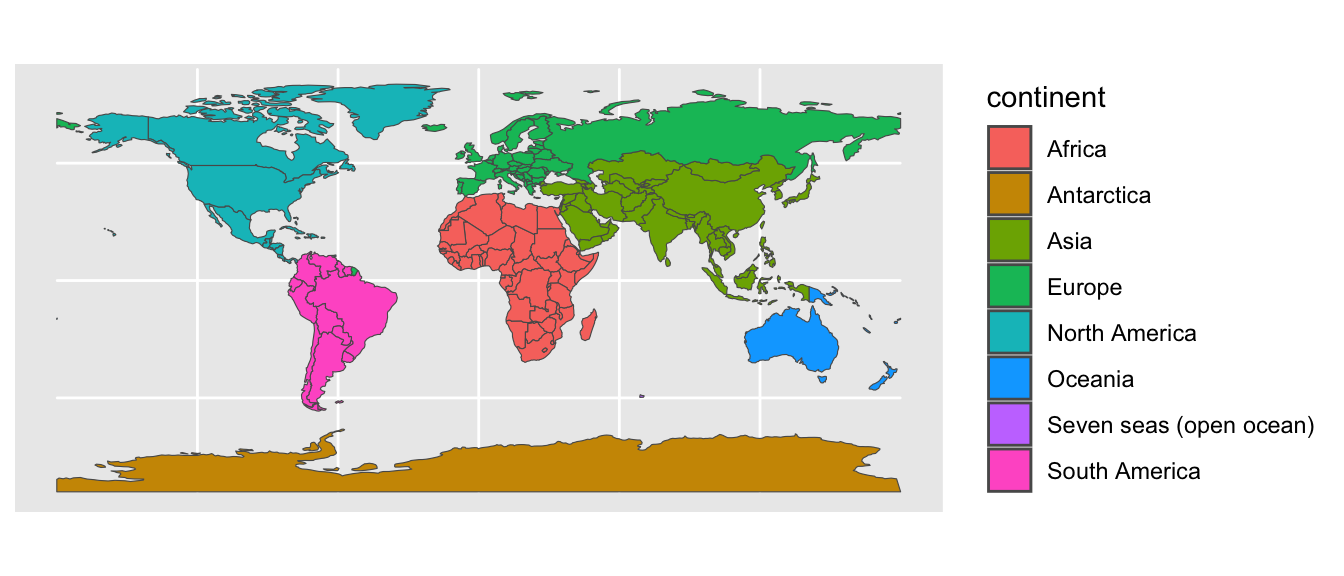

13.1.3 Common Simple-Feature Geometry Types

The types of aesthetics that can be applied to an sf object depend on its geometry type. For example, while fill can be used for polygons, it is not applicable to line strings because, as one-dimensional entities without any area, they cannot be filled with color.

The sf package supports several types of geometries, including points, line strings, and multipolygons. Table 13.1 lists common geometries encountered in practice.

Table 13.1: Common simple-feature geometries

Geometry	Description
POINT	Single coordinate pair
LINESTRING	Sequence of points connected by lines
POLYGON	Object consisting of a sequence of connected line segments that form a closed loop. A polygon is defined by an exterior boundary and zero or more holes.
MULTIPOINT	Set of points, treated as a unit
MULTILINESTRING	Set of line strings, treated as a unit
MULTIPOLYGON	Set of polygons, treated as a unit
GEOMETRYCOLLECTION	Collection of one or more geometries of any type

The following sections introduce the most common types of geometries encountered in practice: points (Section 13.1.3.1), line strings (Section 13.1.3.2), and multipolygons (Section 13.1.3.3).

Common geometry types stored in sf objects are POINT, LINESTRING, and MULTIPOLYGON.

13.1.3.1 Points

A point is the most fundamental geometry type, representing a single coordinate pair. An example of an sf object containing point data is the metro data set from the tmap package. It comprises the locations of 320 large metropolitan areas worldwide. For instance, the code below prints the longitude and latitude of Singapore as a pair of one x-coordinate and one y-coordinate:

The POINT geometry type represents a single coordinate pair.

data(metro, package = "tmap")
metro |>
  filter(name == "Singapore") |>
  st_coordinates()

            X       Y
[1,] 103.8501 1.28967

The st_geometry_type() function from the sf package can be used to determine the geometry type of an sf object. It reveals that the metro data set contains points:

Use st_geometry_type() to identify the geometry type of each row in an sf object.

metro |>
  st_geometry_type() |>
  unique()

[1] POINT
18 Levels: GEOMETRY POINT LINESTRING POLYGON MULTIPOINT ... TRIANGLE

The st_is() function can be used to verify the geometry type of each row in an sf object. For instance, the output below confirms that all rows in the metro data set contain points:

Use st_is() to test the geometry type of each row in an sf object.

metro |>
  st_is("POINT") |>
  all()

[1] TRUE

The following code creates a basic map that shows the points in the metro data set. For spatial context, we also include a background layer of country shapes:

ggplot() +
  geom_sf(data = World, color = "grey") +
  geom_sf(data = metro)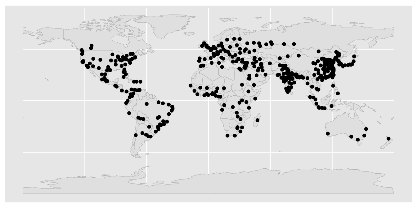

13.1.3.2 Line Strings

A line string is a one-dimensional object composed of a sequence of connected line segments. The World_rivers data set from the tmap package is an example of an sf object that contains line string data. It details the locations of 1,632 major rivers worldwide. For instance, the following code prints the longitude-latitude pairs connected by the Ismailiya Canal:

data(World_rivers, package = "tmap")
World_rivers |>
  filter(name == "Ismailiya Canal") |>
  st_coordinates()

          X      Y L1 L2
[1,] 31.238 30.121  1  1
[2,] 31.282 30.129  1  1
[3,] 31.324 30.180  1  1
[4,] 31.378 30.278  1  1
[5,] 31.483 30.379  1  1
[6,] 31.640 30.484  1  1
[7,] 31.865 30.551  1  1
[8,] 32.303 30.593  1  1

The map below illustrates the content of World_rivers:

The LINESTRING geometry type represents a sequence of connected line segments.

ggplot() +
  geom_sf(data = World, color = "grey") +
  geom_sf(data = World_rivers, color = "navyblue")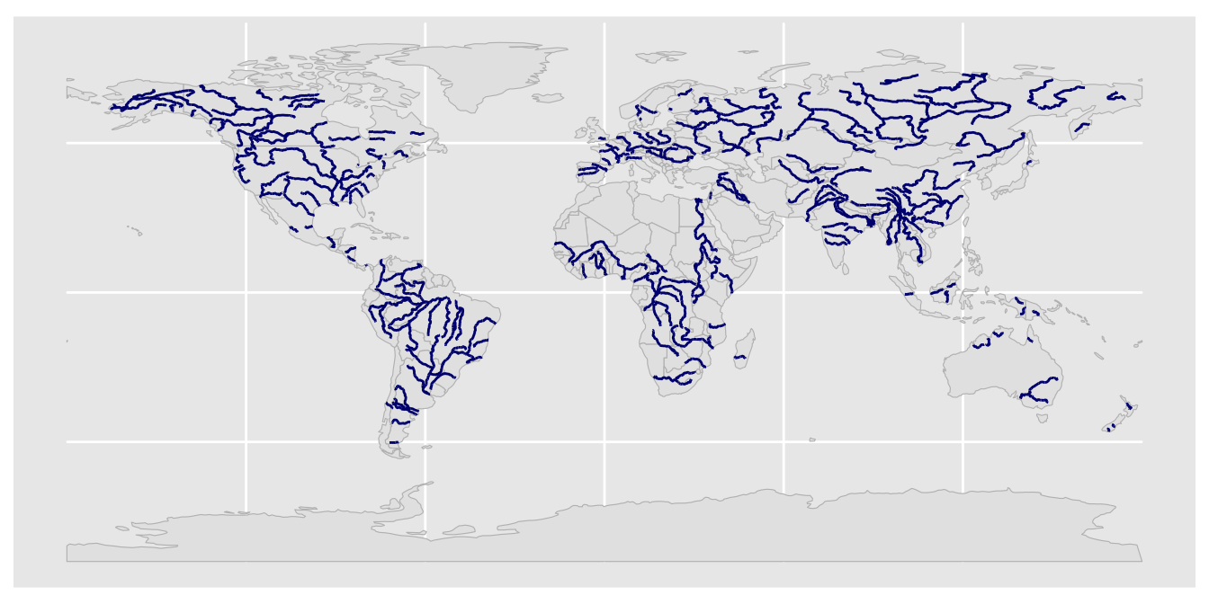

NOTE TO MYSELF: In version >=4.4, tmap’s rivers are Multilinestrings!

13.1.3.3 Multipolygons

A polygon is a two-dimensional object consisting of a sequence of connected line segments that form a closed loop. A multipolygon is defined as a set of polygons that are considered as one entity. For instance, in the World data set, Malaysia is depicted by two polygons—one for Peninsular Malaysia and another for Malaysian Borneo—that are combined into a multipolygon:

The MULTIPOLYGON geometry type represents a set of polygons that are treated as a unit.

mys <- filter(World, name == "Malaysia")
ggplot(mys) +
  geom_sf()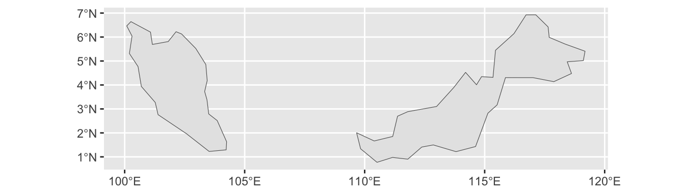

Multipolygons with more than one polygon are common in geospatial data. For instance, regions adjacent to an ocean or a lake are likely to contain several islands, which need to be represented as polygons separate from the mainland.

Additionally, polygons, including those in a MULTIPOLYGON object, can contain holes, which are areas that are excluded from the main body of the polygon. For example, Lesotho is entirely surrounded by South Africa. Hence, Lesotho appears as a hole punched into South Africa:

Polygons can contain holes.

zaf <- filter(World, name == "South Africa")
ggplot(zaf) +
  geom_sf()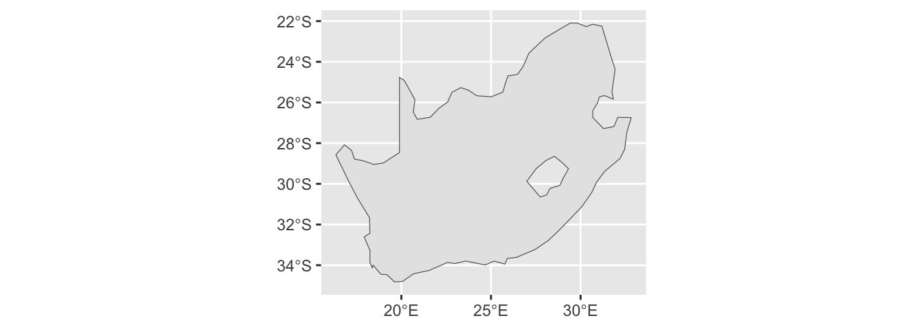

Regions with holes are common in geospatial data because metropolitan regions or capital districts are often represented as holes in the surrounding administrative region. For instance, Kuala Lumpur and Putrajaya are holes in the Malaysian state of Selangor, and Berlin is a hole punched into the German state of Brandenburg.

13.1.4 Importing Geospatial Data as sf Objects

Most examples in this section use pre-installed sf objects. However, in many applications, it is necessary to import geospatial data from a file. The most common file types for geospatial data are GeoJSON (with the extension .json or .geojson) and shapefiles (with the extension .shp).

These and several other geospatial file types can be imported using the read_sf() function from the sf package. To demonstrate the use of read_sf(), please first download the GeoJSON file containing the boundaries of Planning Areas in Singapore from GitHub. Then, move the downloaded file to your current RStudio project directory. The following code imports the file using read_sf():

Use read_sf() to import data from geospatial files, such as GeoJSON and shapefiles.

sgp_pa <- read_sf("singapore_by_planning_area_since_1999.geojson")
sgp_pa

Simple feature collection with 55 features and 5 fields
Geometry type: MULTIPOLYGON
Dimension:     XY
Bounding box:  xmin: 103.6057 ymin: 1.16711 xmax: 104.0882 ymax: 1.470775
Geodetic CRS:  WGS 84
# A tibble: 55 × 6
   shapeName        Level shapeID shapeGroup shapeType                  geometry
   <chr>            <chr> <chr>   <chr>      <chr>            <MULTIPOLYGON [°]>
 1 Ang Mo Kio       ADM2  SGP-AD… SGP        ADM2      (((103.8581 1.391112, 10…
 2 Bedok            ADM2  SGP-AD… SGP        ADM2      (((103.9321 1.305548, 10…
 3 Bishan           ADM2  SGP-AD… SGP        ADM2      (((103.8283 1.367472, 10…
 4 Boon Lay         ADM2  SGP-AD… SGP        ADM2      (((103.6973 1.307544, 10…
 5 Bukit Batok      ADM2  SGP-AD… SGP        ADM2      (((103.7704 1.349016, 10…
 6 Bukit Merah      ADM2  SGP-AD… SGP        ADM2      (((103.8235 1.258507, 10…
 7 Bukit Panjang    ADM2  SGP-AD… SGP        ADM2      (((103.7704 1.349016, 10…
 8 Bukit Timah      ADM2  SGP-AD… SGP        ADM2      (((103.7646 1.332818, 10…
 9 Central Water C… ADM2  SGP-AD… SGP        ADM2      (((103.8188 1.394341, 10…
10 Changi           ADM2  SGP-AD… SGP        ADM2      (((103.9838 1.31668, 103…
# ℹ 45 more rows

Here is a map visualizing the content of the imported data:

ggplot(sgp_pa) +
  geom_sf()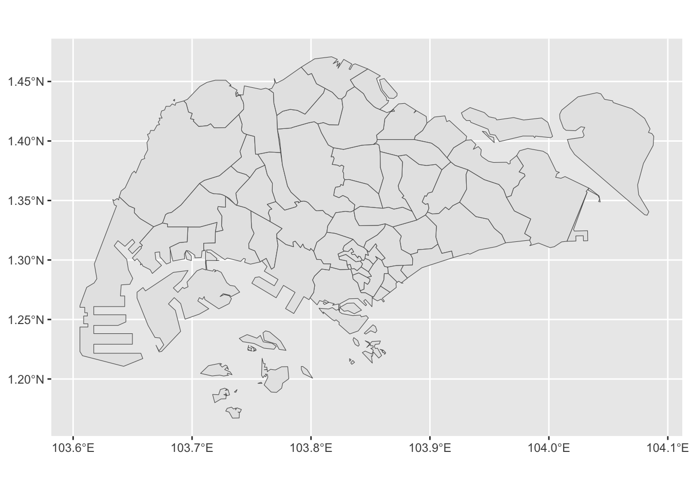

The default settings of read_sf() usually apply reasonable assumptions about the desired geometry types. In this case, the shapes are correctly represented by multipolygons:

sgp_pa |>
  st_geometry_type() |>
  head()

[1] MULTIPOLYGON MULTIPOLYGON MULTIPOLYGON MULTIPOLYGON MULTIPOLYGON
[6] MULTIPOLYGON
18 Levels: GEOMETRY POINT LINESTRING POLYGON MULTIPOINT ... TRIANGLE

In rare cases, it might be necessary to state the desired geometry type explicitly. For example, when called using the type = 5 argument, read_sf() imports the data as multi-line strings. This geometry type would not be suitable in this case because line strings are one-dimensional objects without any area, and, thus, cannot represent the two-dimensional space associated with a planning area:

"singapore_by_planning_area_since_1999.geojson" |>
  read_sf(type = 5) |>
  st_geometry_type() |>
  unique()

[1] MULTILINESTRING
18 Levels: GEOMETRY POINT LINESTRING POLYGON MULTIPOINT ... TRIANGLE

13.1.5 Section Summary

This section introduced sf objects, establishing a framework for working with geospatial data using R. Because all sf objects are also members of the data.frame class, they can be handled using standard tidyverse functions, such as select() and filter(). This chapter also highlighted the geom_sf() function from the ggplot2 package as a tool for visualizing sf objects. Additionally, the chapter discussed three geometry types prevalent in real-world data: points, line strings, and multipolygons. These geometric objects can be imported from external sources using the read_sf() function.

13.2 Handling Common Issues with Geospatial Data

Geometric objects are inherently more complex than tabular data, and this complexity can lead to a variety of issues that need to be addressed before geospatial data can be analyzed or visualized. For instance, geospatial data files frequently contain topological errors, such as overlapping or self-intersecting polygons. Section 13.2.1 demonstrates how to repair these errors. Additionally, files obtained from geospatial data repositories often include more points in line strings and polygons than necessary, causing excessive file sizes and slow rendering speed of the corresponding maps. Section 13.2.2 explains how to reduce the number of points through line simplification.

13.2.1 Repairing Invalid Geometries

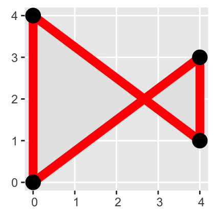
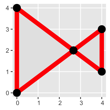
Topological inconsistencies are a common problem in geospatial data sets. For example, polygons may incorrectly overlap or self-intersect, leading to ambiguities in the definition of their interior and exterior. An example of a self-intersection is illustrated in the following figure. The code is for demonstration purposes only and does not need to be memorized:

Overlapping or self-intersecting polygons are common topological errors in geospatial data.

self_intersecting_pgon <-
  rbind(c(0, 4), c(4, 1), c(4, 3), c(0, 0), c(0, 4)) |>
  list() |>
  st_polygon() |>
  st_sfc()
ggplot(self_intersecting_pgon) +
  geom_sf(color = "red", linewidth = 3) +
  geom_sf( # Add points to the plot
    data = st_cast(self_intersecting_pgon, "POINT"),
    size = 5,
    shape = 16 # Filled circles, see ?points
  )

The st_is_valid() function identifies self-intersecting polygons as invalid:

st_is_valid(self_intersecting_pgon)

[1] FALSE

In such cases, using st_make_valid() might be able to convert an invalid polygon into a valid multipolygon by inserting the intersection point as a vertex in two polygons. In the example below, the intersection point is at the coordinates (2.666667, 2):

The st_make_valid() function can often, but not always, repair invalid geometries.

valid_mpgon <- st_make_valid(self_intersecting_pgon)
st_geometry_type(valid_mpgon)

[1] MULTIPOLYGON
18 Levels: GEOMETRY POINT LINESTRING POLYGON MULTIPOINT ... TRIANGLE

st_coordinates(valid_mpgon)

            X Y L1 L2 L3
[1,] 0.000000 4  1  1  1
[2,] 2.666667 2  1  1  1
[3,] 0.000000 0  1  1  1
[4,] 0.000000 4  1  1  1
[5,] 2.666667 2  1  2  1
[6,] 4.000000 3  1  2  1
[7,] 4.000000 1  1  2  1
[8,] 2.666667 2  1  2  1

ggplot(valid_mpgon) +
  geom_sf(color = "red", linewidth = 3) +
  geom_sf(
    data = st_cast(valid_mpgon, "POINT"),
    size = 5,
    shape = 16
  )

While this example was deliberately kept simple, similar issues caused by invalid polygons also arise in real-world data sets. For instance, the GeoJSON file available from GitHub includes invalid polygons. It contains boundaries of subzones in Singapore, which tend to be smaller than the planning areas plotted in the previous chapter. The subzone boundaries were obtained from Data.gov.sg (2024):

subzones <- read_sf("singapore_subzones.geojson")
all(st_is_valid(subzones))

[1] FALSE

As before, you can use the st_make_valid() function to rectify the invalid geometries:

subzones <- st_make_valid(subzones)
all(st_is_valid(subzones))

[1] TRUE

The following code chunk visualizes the repaired polygons:

gg_subzones <-
  ggplot(subzones) +
  geom_sf()
gg_subzones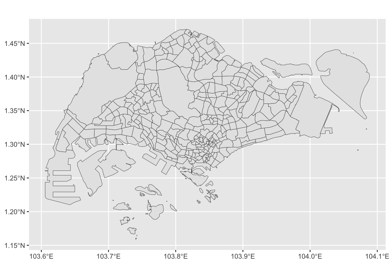

13.2.2 Simplifying Line Strings and Polygons

Geospatial boundaries stored in online data repositories often include an excessive number of points in line strings and polygons. A general rule of thumb is that maps typically do not require more than 10,000 boundary points. The number of boundary points can be determined using the npts() function from the mapview package. It indicates that the number of points in the previous map exceeds the target value of 10,000:

library(mapview)
npts(subzones)

[1] 58797

The ms_simplify() function in the rmapshaper package can effectively reduce the number of points in geospatial data:

Use ms_simplify() from the rmapshaper package to reduce the number of points in line strings and polygons.

library(rmapshaper)
simplified <- ms_simplify(subzones)
npts(simplified)

[1] 5308

The following code places the original and simplified maps side by side, enabling an easy comparison between them:

gg_subzones
ggplot(simplified) +
  geom_sf()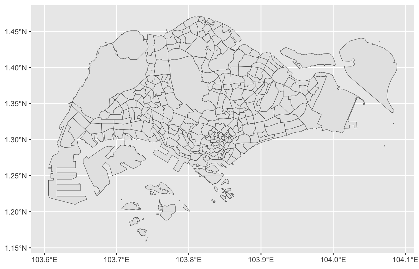

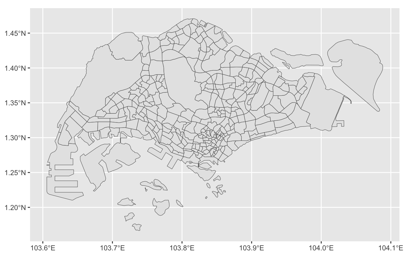
A few islands and some details of the shapes have been removed by the simplification. However, overall, the differences between the two maps are barely visible. As this example demonstrates, simplifying the boundary can significantly reduce the number of points, resulting in faster calculations and quicker rendering of the graphic, while maintaining almost the same visual appearance.

13.2.3 Section Summary

Searching for geospatial data can be challenging. Some useful data repositories include GADM, the World Bank, and government web sites, such as the US Census Bureau and Data.gov.sg. After importing the data, it is advisable to check for invalid geometries using the st_is_valid() function and, if necessary, repair them using the st_make_valid() function. Finally, the ms_simplify() function from the rmapshaper package can be used to reduce the number of points in line strings and polygons, which can decrease both the file size and the rendering speed of the visualization.

13.3 Map Projections

The Earth’s surface is approximately spherical, which means that any geographic map displayed on a flat, two-dimensional surface must be a transformation of the actual spatial relationships. Such a transformation is known as a map projection. Gauss’s Theorema Egregium states that there is no distortion-free map projection that can flatten a sphere. Due to the absence of an ideal, distortion-free projection, past centuries witnessed the proposals of numerous projections that reduce distortions in various ways, each serving different purposes. A gallery of map projections can be found on Wikipedia.

A map projection is a geographic transformation that converts a position on the surface of the Earth to a position on a flat map.

Map projections are encoded using a Coordinate Reference System (CRS), which specifies a set of parameters that define the projection method. These parameters can be retrieved for a given sf object using the st_crs() function. The information returned by st_crs() includes the projection’s name and the Spatial Reference System Identifier (SRID), which is a unique identifier for a map projection assigned by the Open Geospatial Consortium. For instance, the World object from the tmap package uses the SRID “EPSG:4326”:

A Coordinate Reference System (CRS) specifies the type and parameters of a map projection.

library(tmap)
data(World)
st_crs(World, parameters = TRUE)$srid

[1] "EPSG:4326"

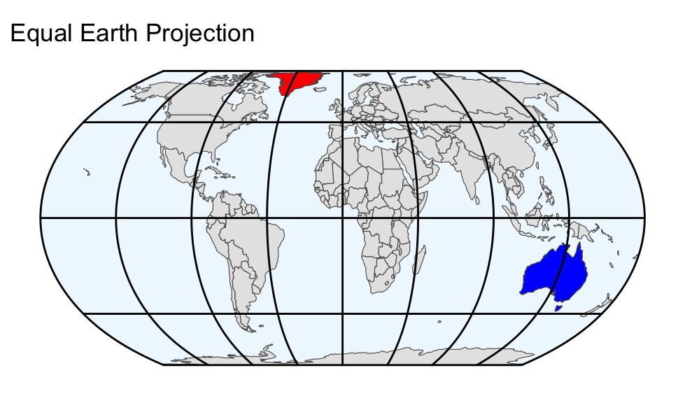
When plotting an sf object using EPSG:4326, longitude is, by default, mapped to the x-coordinate and latitude to the y-coordinate, as shown in Figure 13.1. Because lines of constant longitude and latitude intersect at right angles on the map, and latitude differences are scaled proportionally into y-coordinate differences, this projection is referred to as “equirectangular.” Although algorithmically straightforward, the equirectangular projection significantly distorts areas and shapes. For example, Greenland (highlighted in red) appears comparable in area to Australia (highlighted in blue) on the map; however, in reality, it has only 28% of Australia’s land area. Additionally, Greenland is substantially stretched in the east-west direction compared to its true shape on the globe:

The equirectangular projection is a simple projection that maps longitude to the x-coordinate and latitude to the y-coordinate. However, areas on the map do not represent surface areas in correct proportion.

gg_world <- ggplot(World) +
  geom_sf() +
  geom_sf(
    aes(fill = name),
    data = filter(World, name %in% c("Greenland", "Australia"))
  ) +
  scale_fill_manual(values = c("Greenland" = "red", "Australia" = "blue")) +
  guides(fill = "none") +
  theme(
    panel.background = element_blank(),
    panel.grid = element_line(color = "black"),
    panel.ontop = TRUE
  )
gg_world + labs(title = "Equirectangular Pojection")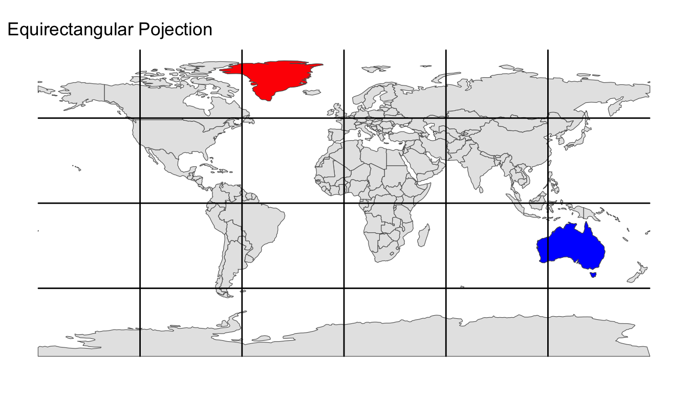

Figure 13.1: The Earth in an equirectangular projection. Greenland and Australia are highlighted in red and blue, respectively.

For choropleth maps, which are the focus of Section 13.4, the equirectangular projection is suboptimal because the area on the map is uninterpretable as a data value. Instead, it is preferable to choose an equal-area projection (i.e., a projection that faithfully represents area proportions). There are various equal-area projections available, for example:

An equal-area projection is a map projection that accurately preserves the relative sizes of areas on the Earth’s surface.

• Sinusoidal projection (SRID ESRI:54008)
• Mollweide (SRID ESRI:54009)
• Eckert IV projection (SRID ESRI:54012)
• Behrmann projection (SRID ESRI:54017)
• Equal Earth projection (SRID ESRI:54035)

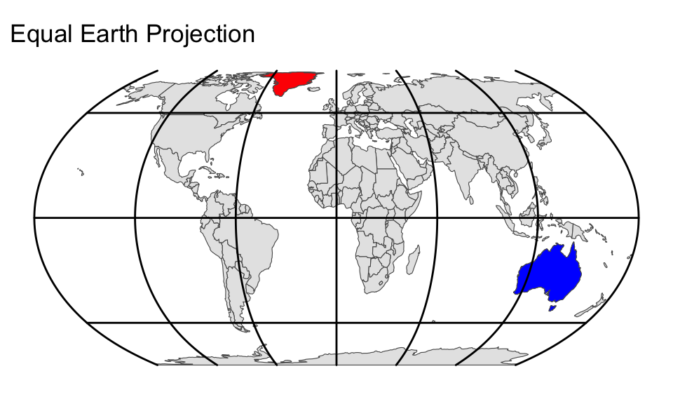
To project an sf object, ggplot2’s coord_sf() function can be used with the crs argument equal to the chosen SRID. The following code chunk demonstrates how to transform the World object using the Equal Earth projection. The resulting map is then shown alongside the equirectangular projection. Greenland and Australia are highlighted in red and blue, respectively. Note that, in the Equal Earth projection, the areas of Greenland and Australia are represented in correct proportion:

Use coord_sf() to project an sf object into a different map projection.

gg_world + labs(title = "Equirectangular Pojection")
gg_world +
  coord_sf(crs = "ESRI:54035") +
  labs(title = "Equal Earth Projection")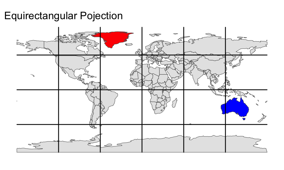

To highlight the projected nature of the maps, it is advisable to indicate the boundaries of the projected Earth. The following code defines an sf object named earth, which encompasses the entire globe. The syntax might appear complex and does not need to be memorized. However, it is noteworthy that the coordinates are entered as longitude and latitude, with \(\pm\) 180 representing the longitudes of the antimeridians, and 90 and -90 representing the latitudes of the North and South Poles, respectively. Five different equal-area projections are plotted alongside the equirectangular projection to illustrate the variations. The projected longitude-latitude graticules are overlaid to facilitate comparison between the map projections:

earth <- st_polygon(
  x = list(
    cbind(
      c(rep(-180, 181), rep(180, 181), -180), c(-90:90, 90:-90, -90)
    )
  )
) |>
  st_sfc() |>
  st_set_crs(4326) |> # Equirectangular projection
  st_as_sf()
gg_world_boundary <-
  ggplot(World) +
  geom_sf(data = earth, fill = "aliceblue") +
  geom_sf() +
  geom_sf(
    aes(fill = name),
    data = filter(World, name %in% c("Greenland", "Australia"))
  ) +
  scale_x_continuous(breaks = seq(-180, 180, by = 45)) +
  scale_y_continuous(
    breaks = c(-89.9, -45, 0, 45, 89.9) # Avoid singularities at +/-90
  ) +
  scale_fill_manual(values = c("Greenland" = "red", "Australia" = "blue")) +
  guides(fill = "none") +
  theme(
    panel.background = element_blank(),
    panel.grid = element_line(color = "black"),
    panel.ontop = TRUE
  )
gg_world_boundary + labs(title = "Equirectangular Pojection")
gg_world_boundary +
  coord_sf(crs = "ESRI:54008") +
  labs(title = "Sinusoidal Projection")
gg_world_boundary +
  coord_sf(crs = "ESRI:54009") +
  labs(title = "Mollweide Projection")
gg_world_boundary +
  coord_sf(crs = "ESRI:54012") +
  labs(title = "Eckert IV Projection")
gg_world_boundary +
  coord_sf(crs = "ESRI:54017") +
  labs(title = "Behrmann Projection")
gg_world_boundary +
  coord_sf(crs = "ESRI:54035") +
  labs(title = "Equal Earth Projection")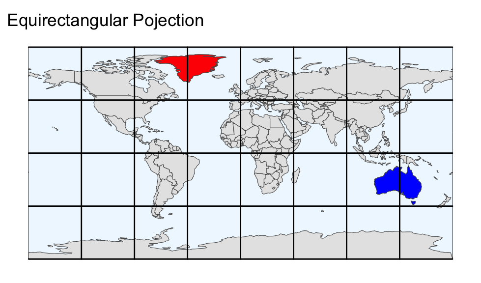

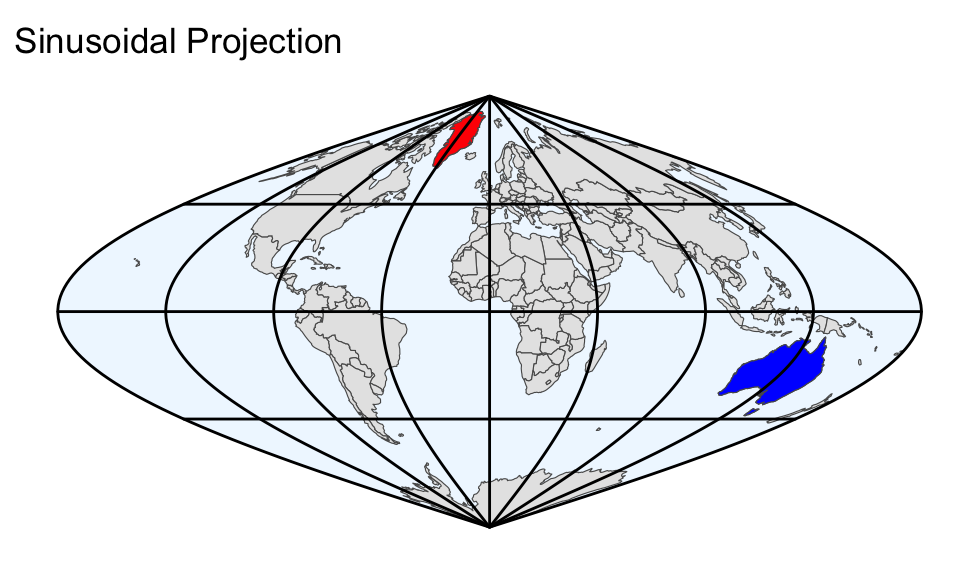
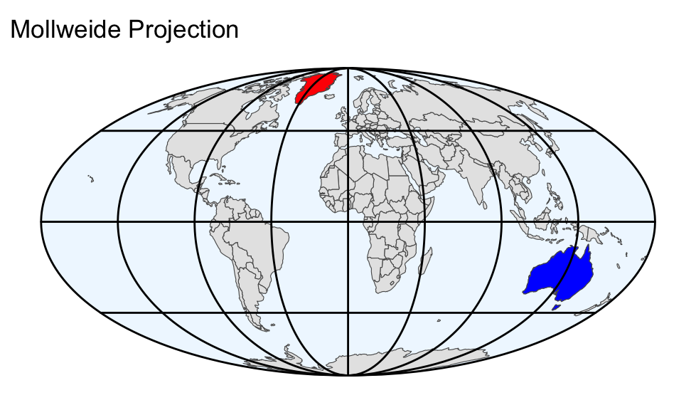
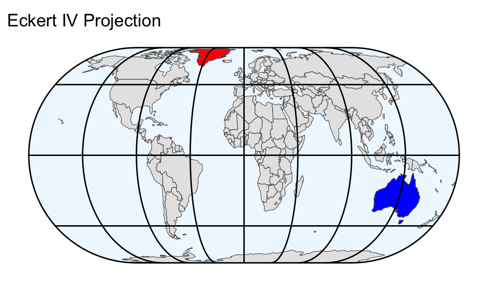
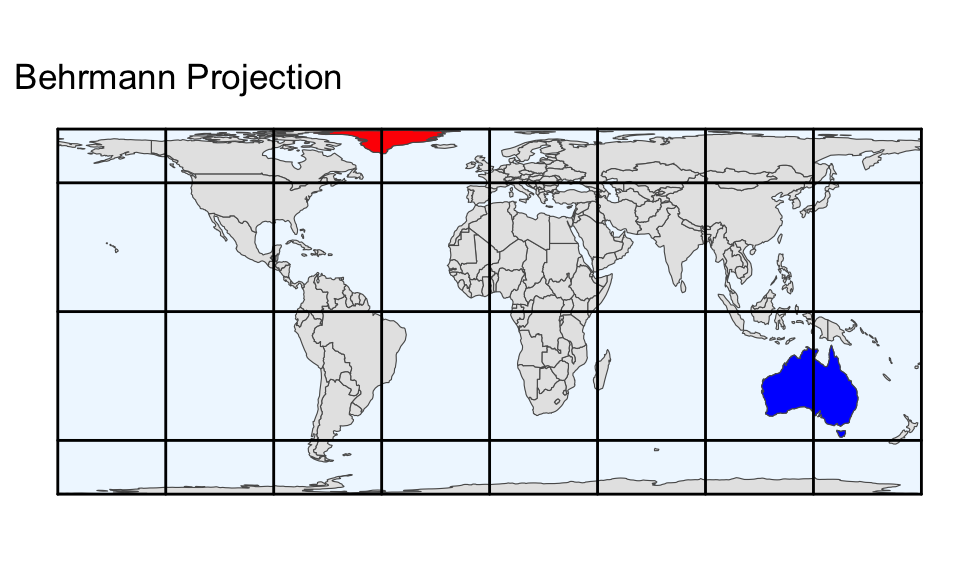
Comparing the equal-area projections in the output above, the most noticeable difference is the shape of the Earth’s boundary:

Equal-area projections vary in the way they depict the poles and the boundaries of the projected Earth.

Sinusoidal projection:

The poles are correctly depicted as single points. The eastern and western antimeridian meet at the poles, forming a sharp corner.

Mollweide projection:

Similar to the sinusoidal projection, but the antimeridians merge into each other without any sharp corners at the poles.

Eckert IV projection:

The poles are stretched into horizontal lines but are shorter than the equator. Representing the poles as lines is in stark contrast with reality, where they are points without any length. The Eckert IV projection depicts both antimeridians as curved, smoothly merging into the pole lines without any sharp corners.

Behrmann projection:

The poles are stretched into horizontal lines and all parallels (i.e., lines of constant latitude) are equally long.

Equal Earth projection:

Similar to the Eckert IV projection, but the antimeridians meet the pole lines at an obtuse angle.

While it is advisable to select an equal-area projection for choropleth maps, there is no simple rule for choosing the right map projection. The Eckert IV and Equal Earth projections are both viable options if stretching the poles into lines is acceptable. Otherwise, the Mollweide projection is a suitable alternative.

For a light-hearted perspective on map projections, please have a look at the cartoon by Munroe (2011) at https://xkcd.com/977/. Based on this cartoon, which map projection type do you identify with?

13.4 Choropleth Maps

A map is called choropleth (derived from the ancient Greek words χῶρος for area and πλῆθος for multitude) if it satisfies all of the following criteria:

• The variable to be visualized consists of one number per region.

• Regions do not overlap.

• Regions are filled with colors that represent the variable.

• Regions are determined before data are collected. In other words, regions are not established retrospectively from the data. For example, the world’s land masses might be divided into countries before data (e.g., on life expectancy or gross domestic product) for each country are collected and aggregated (e.g., by taking the mean).

  In contrast, a map that visualizes land cover (i.e., the physical material on the surface of the earth, such as forest, grassland, or asphalt) by polygons of different colors is generally not a choropleth map because the polygon boundaries are only known after data are collected. Instead, such a map is called dasymetric.

• The variable is an intensive quantity, as defined in Section 8.1.2. That is, the variable is not expected to depend significantly on a region’s size (e.g., measured in terms of spatial extent or total population). Intensive variables often belong to one of the following types:

  1. The ratio of two additive variables. A variable is additive if its value for a larger region is the sum of the values of its subregions. For example, GDP or population are additive. Hence, GDP per capita is a suitable variable to be depicted by color on a choropleth map because it is the ratio of the GDP to the population.
  2. The proportion or percentage of a subset of observations to the total number of observations (e.g., the percentage of unemployed individuals in the population).
  3. Spatial density measured in units of inverse area (e.g., the number of solar panels per square kilometer).
  4. The rate of change in percent (e.g., the increase in GDP from one year to the next).

In this chapter, you will build choropleth maps that visualize the number of automated teller machines (ATMs) per 100,000 adults in 2021 by country. This variable belongs to type 1 in the list above because both the number of ATMs and the population in 100,000 are approximately proportional to area. The data, downloaded from the World Bank on the 11th of June 2024, are available from GitHub. You can download the data and merge it with the geospatial country boundaries contained in tmap’s World object as follows:

Use choropleth maps only for intrinsic ordinal or intensive quantitative variables.

library(tmap)
data(World)
atm <-
  "atm.xls" |>
  readxl::read_xls(skip = 3) |>
  select(
    country = `Country Name`,
    code = `Country Code`,
    atm_2021 = `2021`
  )
world <-
  World |>
  left_join(atm, by = c("iso_a3" = "code")) |>
  select(country, code = iso_a3, area, atm_2021)

The following sections will:

• discuss suitable palettes (Section 13.4.1),
• explain how missing values can be added to the legend (Section 13.4.2).
• demonstrate how to label the largest countries on the map (Section 13.4.3).

13.4.1 Choosing a Suitable Palette

A crucial step in creating a choropleth map is setting the fill aesthetic equal to the intensive variable of interest. In the following map, the fill aesthetic is determined by the atm_2021 column of the world object. The map applies the Equal Earth projection, draws the boundaries of the projected Earth, and fills oceans with a light blue color:

Choropleth maps require the fill aesthetic to be set to an intensive statistical variable.

earth <- st_polygon(
  x = list(
    cbind(
      c(rep(-180, 181), rep(180, 181), -180), c(-90:90, 90:-90, -90)
    )
  )
) |>
  st_sfc() |>
  st_set_crs(4326) |> # Equirectangular projection
  st_as_sf()

gg_atm_2021 <-
  ggplot() +
  geom_sf(data = earth, fill = "lightblue1") +
  geom_sf(aes(fill = atm_2021), data = world, color = "black") +
  labs(
    fill = NULL,
    title = "Automated Teller Machines per 100,000 Adults in 2021"
  ) +
  coord_sf(crs = "ESRI:54035") +
  theme_void() +
  theme(
    legend.margin = margin(5, 0, 0, 0), # Increase margin above legend
    legend.key.width = unit(1.25, "cm"),
    legend.frame = element_rect(), # Add a frame around the colorbar
    legend.position = "top",
    plot.title = element_text(face = "bold", hjust = 0.5),
  )
gg_atm_2021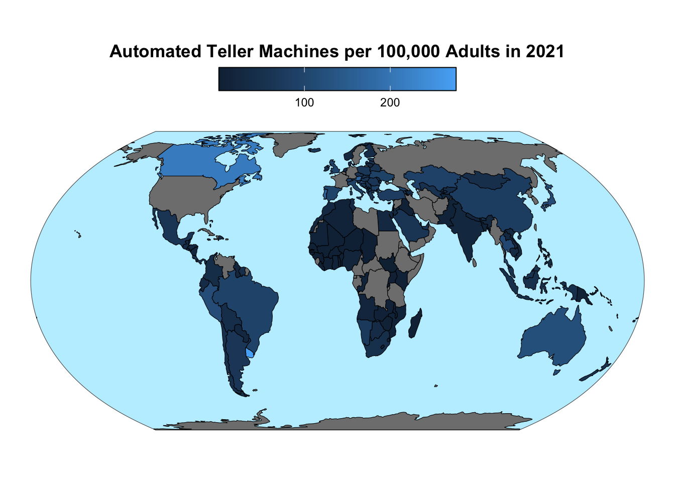

The default palettes of ggplot are generally not the best choices for choropleth maps. As discussed in a previous lesson, the palettes from the ColorBrewer website, produce more effective visualizations. These palettes are accessible through ggplot2’s scale_fill_fermenter() function for ordinal and quantitative data. If the data are nominal, you can use scale_fill_brewer() instead.

Use scale_fill_fermenter() or scale_fill_brewer() to apply a ColorBrewer palette to a choropleth map.

You need to carefully consider the type of palette suitable for the variable you are depicting. Here is a recap of your earlier lesson on choosing colors:

• You should opt for a sequential palette if the variable is non-negative and either ordinal or quantitative. Additionally, when displayed on a white background, lighter colors should represent smaller values.

• For variables that include both positive and negative values, a diverging palette is the appropriate choice. The lightest color in the palette should represent the value zero.

• For nominal variables, you should use one of ColorBrewer’s qualitative palettes. They are specifically designed to distinguish data without a natural order or ranking. Each category is represented by a distinct color, making it easier to differentiate between them visually.

Use a sequential palette for non-negative variables. Use lighter colors to represent smaller values.

Use a diverging palette for variables with both positive and negative values. Place the lightest color at zero.

Use a qualitative palette for nominal variables.

The atm_2021 variable, being constrained to non-negative values, calls for a sequential palette. Additionally, the palette should contrast with the blue color of the oceans. The code below applies the Greens palette from ColorBrewer and light gray for missing values. A logarithmic scale is used because atm_2021 is right-skewed (i.e., most values are at the low end of the range, but a few are larger by more than a factor of 10):

gg_atm_2021 <-
  gg_atm_2021 +
  scale_fill_fermenter(
    breaks = scales::breaks_log(n = 6),
    palette = "Greens",
    direction = 1,
    na.value = "gray80"
  )
gg_atm_2021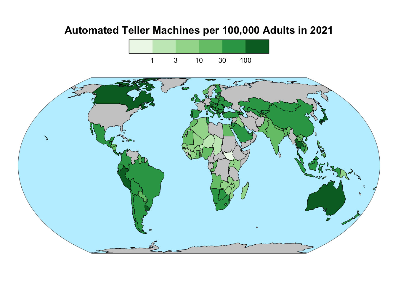

13.4.2 Adding Missing Values to the Legend

The colorbars provided by ggplot2 omit a legend entry for missing values, potentially confusing readers about the nature of the off-palette data value. To address this issue, you can add a legend entry for missing values by setting the color aesthetic to a constant value, as implemented by the code below. The fill color of this legend entry is set to the same color, gray80, as the missing values in the map. Additionally, the order argument of the guide_*() functions is used to shift the missing value from the start to the end of the legend, following the conventional order:

Add a legend entry for missing values by first setting the color aesthetic to a constant value. Then, use guide_legend() to fill the legend with the desired color.

gg_atm_2021 <-
  gg_atm_2021 +
  aes(color = NA) +
  guides(
    fill = guide_colorsteps(order = 1),
    color = guide_legend(override.aes = list(fill = "gray80"), order = 2)
  )
gg_atm_2021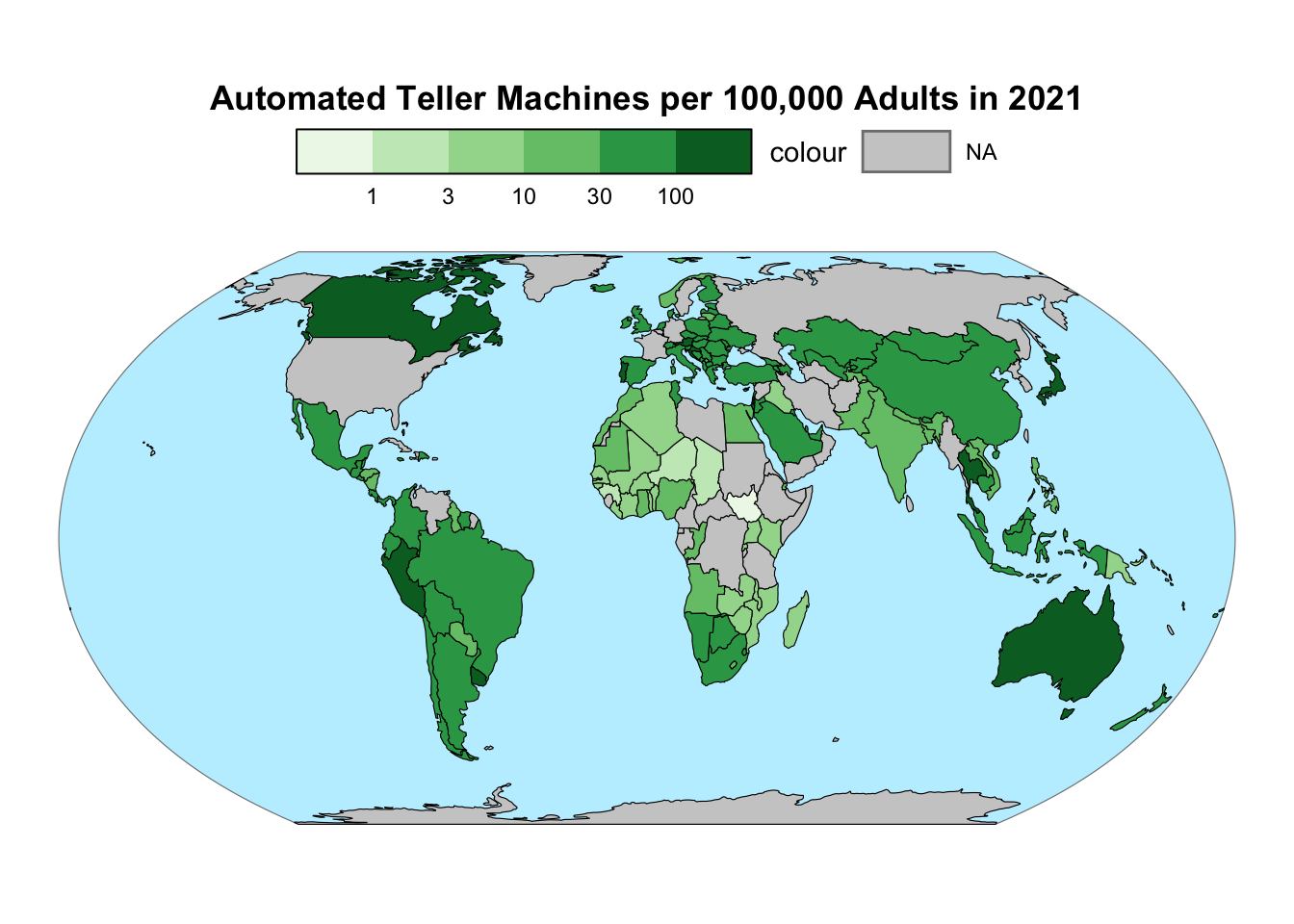

To fine-tune the legend, the “colour” title should be removed. Additionally, the “NA” label ought to be replaced by the more descriptive term “Missing”, while also placing it at the bottom of the legend:

gg_atm_2021 <-
  gg_atm_2021 +
  labs(color = NULL) +
  scale_color_manual(labels = "Missing", values = "black") +
  theme(legend.text.position = "bottom")
gg_atm_2021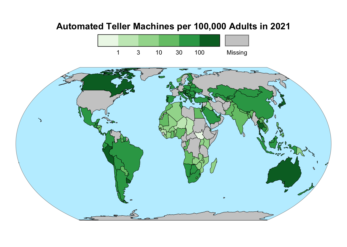

13.4.3 Adding Labels

To improve the readability of a choropleth map, it is advisable to label at least the largest geographic units. This task can be accomplished using ggplot2’s geom_sf_text() function. The code below adds the three-letter codes of the twenty largest countries as labels, taking advantage of the area column that was included in the original World object. If the area is not part of the original data, it can be calculated using the st_area() function from the sf package. The label color should be chosen such that it provides a clear contrast against the background color (e.g., black on light-colored backgrounds but white on dark-colored ones):

gg_atm_2021 <-
  gg_atm_2021 +
  geom_sf_text(
    aes(label = code),
    data = filter(
      world,
      min_rank(desc(area)) <= 20 & (is.na(atm_2021) | atm_2021 <= 30)
    ),
    color = "black",
    size = 1.7
  ) +
  geom_sf_text(
    aes(label = code),
    data = filter(
      world,
      min_rank(desc(area)) <= 20 & atm_2021 > 30
    ),
    color = "white",
    size = 1.7
  )
gg_atm_2021

13.4.4 Section Summary

In this chapter, you learned how to use ggplot2 for crafting choropleth maps that meet professional cartographic standards. The chapter reiterated the importance of selecting an appropriate palette. Additionally, it demonstrated how to include a legend entry for missing values and incorporate labels for clarity. These skills will enable you to present geospatial data effectively, ensuring that your maps are both informative and visually appealing.

13.5 Conclusion

This chapter introduced you to fundamental skills required for geospatial data visualization. It highlighted the features of the sf class, which provides a convenient interface for working with geospatial data in R. You learned how to import geospatial data using the read_sf() function, repair topological errors, and simplify geometries to accelerate rendering and decrease file sizes. You also learned how to create choropleth maps, which are the most common map type for visualizing geospatial data. However, it is crucial to note that the variable displayed by choropleth maps must be intensive. For non-intensive data, other map types are required, such as proportional-symbol maps and cartograms.

While ggplot2 is a powerful tool, there are more specialized R packages for map creation. If you require more advanced mapping capabilities, consider exploring the tmap package, which, like ggplot2, adheres to grammar-of-graphics principles (Tennekes, 2018). However, unlike ggplot2, tmap adds missing values automatically to legends and provides more user-friendly options for labeling regions.

Exercise

The ATM data on GitHub include both years 2020 and 2021. Create a choropleth map visualizing the percentage change in the number of ATMs per 100,000 adults between these two years. Which type of palette should be chosen?

Data.gov.sg (2024) Master Plan 2019 Subzone Boundary (No Sea) (GEOJSON). Available at: https://data.gov.sg/dataset/master-plan-2019-subzone-boundary-no-sea-geojson (Accessed: June 14, 2024).

Munroe, R. (2011) Map Projections, xkcd. Available at: https://xkcd.com/977/ (Accessed: March 28, 2022).

Tennekes, M. (2018) “Tmap: Thematic maps in r,” Journal of Statistical Software, 84(6), pp. 1–39. Available at: https://doi.org/10.18637/jss.v084.i06.

---

1. In principle, the geometry column can be renamed, for example, using the rename() function from the dplyr package. In that case, the sf_column attribute of the sf object is automatically updated to reflect the new name. However, in practice, renaming the geometry column is not recommended because it might lead to confusion.