stars object with 2 dimensions and 1 attribute
attribute(s):
                  Min.  1st Qu.   Median     Mean  3rd Qu.     Max.
elevation [m] 1832.444 2540.651 2846.281 2843.889 3118.472 4330.093
dimension(s):
  from  to offset      delta refsys point x/y
x    1 467  7.594  0.0002778 WGS 84 FALSE [x]
y 1 325 46.02 -0.0002778 WGS 84 FALSE [y]17 Visualizing Geospatial Rasters
The previous chapter showed how to map geospatial vector data: points, lines, and polygons, each recorded as explicit coordinates. This chapter turns to the other main class of geospatial data: rasters. Instead of storing coordinates for every observation, a raster arranges values on a regular grid, so each cell’s position follows from the grid’s origin and cell size. Figure 17.1 illustrates the difference by showing the same landscape both ways: The river is a crisp polyline in the vector data displayed on the left but appears coarse-grained in the raster data on the right. Vector data suit discrete objects with clearly defined boundaries or paths; rasters suit spatially varying measurements (e.g., elevation) and classifications (e.g., land cover). In this chapter, we import, inspect, and visualize rasters with the stars package and ggplot2.
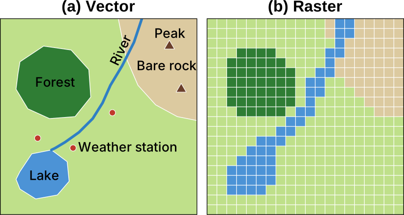
Section 17.1 introduces this chapter’s running example: raster data for the Matterhorn region. The remaining sections align with the typical raster-data workflow:
- Loading: Section 17.2
- Inspecting: Sections 17.3 and 17.4
- Geoprocessing: Sections 17.5–17.8
- Communicating visually: Sections 17.9–17.10
17.1 A First Raster Map: Matterhorn Region
Before examining how rasters are structured, it helps to see how to move from a raster file to a map using a minimal example. The example uses a digital elevation model (DEM) of the Matterhorn region, cropped to a 10 km by 10 km square on the Swiss–Italian border and taken from the Copernicus DEM GLO-30 product.1 Each cell records the surface elevation, in meters. The following code reads the file:
The read_stars() function loads a GeoTIFF file into a stars object, which combines attributes and dimensions. In this example, elevation is the only attribute, while x and y are the dimensions. By default, the attribute would take the name of the input file; to ensure a concise, meaningful attribute name, we set it to elevation using setNames(). The output also summarizes the attribute’s values, showing that elevation ranges from about 1,800 m in the valleys to roughly 4,300 m near the summit. From the band metadata stored in the GeoTIFF, read_stars() knew that height is measured in meters ([m]).
Additionally, the output provides the spatial information needed to place the cells on the Earth’s surface:
-
fromandto: the index bounds within the reference grid for each dimension -
offset: the coordinate at the start of cell 1 in the reference grid -
delta: the signed spacing between adjacent cells -
refsys: the coordinate reference system (CRS) used to interpret each dimension -
point: a Boolean value indicating whether positions along a dimension represent points (TRUE) or rectangular intervals (FALSE) -
x/y: which dimensions act as the spatial x- and y-axes, marked by[x]and[y]
The geom_stars() function draws a map of a stars object. Because matterhorn_dem has only one attribute (elevation), geom_stars() maps it to the fill aesthetic automatically. As with other geoms, the colors can be customized with a compatible scale_fill_*() function; for now, we use ggplot2’s default continuous fill scale:
ggplot() +
  geom_stars(data = matterhorn_dem) +
  coord_sf(crs = st_crs(matterhorn_dem)) +
  labs(
    x = "Longitude",
    y = "Latitude",
    fill = "Elevation (m)"
  ) +
  theme_minimal()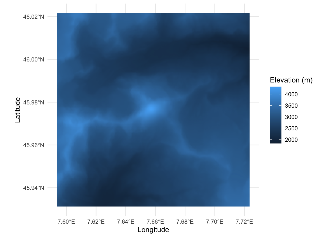
That is the whole recipe: read_stars() to load and geom_stars() to draw. The coord_sf() call is also needed because, unlike sf objects, stars objects do not pass their CRS to the ggplot object. Knowing the CRS, ggplot2 can set the aspect ratio of the map: At the latitude of the Matterhorn, one degree of longitude covers only about 70% of the distance of one degree of latitude. Later sections in this chapter refine these steps.
17.2 Importing a Raster as a stars Object
The preceding section passed a filename to read_stars() and immediately produced a map. We now look more closely at what the file contains, how read_stars() interprets it, and how we can inspect a large raster without immediately loading all its cell values into memory.
17.2.1 GeoTIFF and Other Raster Formats
The Matterhorn elevation data are stored in a file whose name ends in .tif. This extension identifies the Tagged Image File Format (TIFF), commonly used for raster images, such as photos or document scans. When a TIFF also contains the information needed to place its cells geographically, it is called a GeoTIFF.
In addition to the raster values, a GeoTIFF can record metadata such as:
- The CRS
- The spatial extent
- The cell size
- Descriptions and units for individual bands
- The value used to represent missing data
Consolidating the values and their spatial metadata in a single file makes GeoTIFF a convenient, robust format for exchanging geospatial rasters.
GeoTIFF is widely used, but it is only one of several common raster formats. Many environmental datasets—especially those with a time dimension—are stored in Network Common Data Form (NetCDF) files, which use the .nc extension. Other common formats include GRIB for weather and atmospheric data, HDF5 for large scientific datasets, JPEG 2000 for compressed satellite imagery, and ASCII Grid for simple text-based grids.
These formats differ in what they can store and how they organize the stored data. Fortunately, we do not need a different R function for each one. The stars package delegates file access to the Geospatial Data Abstraction Library (GDAL). GDAL provides drivers that understand the individual formats, allowing read_stars() to provide a common interface in R. If an input file declares a NoData value, read_stars() normally converts occurrences of that value to NA.
17.2.2 Lazy Loading with a Proxy
The Matterhorn DEM contains only 467 × 325 cells, so reading all its values into memory is inexpensive. Full national and global datasets can be several orders of magnitude larger. For such files, it is more efficient to inspect and subset the raster before reading all its values.
Setting proxy = TRUE creates a reference to the raster without immediately loading its complete array of cell values:
matterhorn_dem_proxy <- read_stars(
  "matterhorn_dem_copernicus_glo30_native.tif",
  proxy = TRUE
) |>
  setNames("elevation")
matterhorn_dem_proxy
stars_proxy object with 1 attribute in 1 file(s):
$elevation
[1] "matterhorn_dem_copernicus_glo30_native.tif"
dimension(s):
from to offset delta refsys point x/y
x 1 467 7.594 0.0002778 WGS 84 FALSE [x]
y 1 325 46.02 -0.0002778 WGS 84 FALSE [y]The result is a stars_proxy object. Its printed output identifies the source file and describes the raster dimensions, extent, resolution, and CRS. Unlike the printed in-memory object matterhorn_dem in the preceding section, the proxy does not report a statistical summary of the elevation values because those values have not yet been read from disk.
A proxy stores information about where the values can be obtained and records certain operations without carrying them out immediately. For example, we can crop a proxy to a smaller area while it remains a proxy. Reading is deferred until an operation requires the values.
To load the values explicitly, pass the proxy to st_as_stars(). The deferred read is then executed, the array is loaded into memory, and the result becomes an ordinary in-memory stars object:
matterhorn_dem_in_memory <- st_as_stars(matterhorn_dem_proxy)
identical(matterhorn_dem, matterhorn_dem_in_memory)
[1] TRUEIn summary:
- With
proxy = FALSE,read_stars()reads the raster values into memory immediately. - With
proxy = TRUE, it returns astars_proxycontaining metadata and a reference to the source. - The
st_as_stars()function materializes a proxy by reading the required values.
When proxy is not set explicitly, read_stars() compares the number of cells with a size threshold and returns a proxy for larger inputs. Explicitly supplying TRUE or FALSE makes the intended behavior clearer.
A proxy offers no practical advantage for our small Matterhorn DEM, so the remainder of the chapter continues to use the in-memory matterhorn_dem object.
17.3 Attributes and Dimensions
To work with stars objects effectively, we must understand their structure. A stars object is a data cube—one or more arrays of values organized along labeled dimensions:
- Attributes contain the values being represented, such as elevation, temperature, or land-cover class;
- Dimensions describe how those values are organized, for example across space, spectral bands, or time.
The names() function returns the name of its single attribute, elevation, while dim() reports the lengths of its two dimensions, x and y:
The attribute can be extracted using the $ operator or dplyr::pull(). It is stored in an array with the same dimension as the stars object:
elevation_values <- matterhorn_dem$elevation
dim(elevation_values)
x y
467 325 A stars object can contain several attributes that share the same dimensions. For example, an object might contain separate attributes named elevation and temperature, each represented by a 467-by-325 array over the same spatial grid.
Dimensions can also extend beyond the two spatial axes. Consider the three-band Sentinel-2 image supplied with this chapter:2
matterhorn_rgb <- read_stars(
  "matterhorn_rgb_sentinel2_native.tif"
) |>
  setNames("rgb")
dim(matterhorn_rgb)
x y band
1020 1020 3 The object has dimensions x, y, and band. The first two identify a spatial cell; the third selects its red, green, or blue channel. A single cell therefore contains three values:
All three values describe the same patch of ground. They differ systematically by color channel, so representing the channel as a band dimension produces one 1020-by-1020-by-3 array.
The same data could, in principle, be represented by three attributes named red, green, and blue, each arranged over x and y. The band representation reflects the organization of the multiband GeoTIFF and makes it convenient to select, compare, or combine channels along one dimension.
This distinction suggests a useful rule of thumb. Conceptually different quantities measured over the same grid, such as elevation and temperature, are often represented as separate attributes. Values that differ along a systematic axis, such as spectral channel or observation time, are often represented as positions along an additional dimension. The most useful representation depends partly on how the data are stored and how we intend to analyze them.
In short, attributes and dimensions answer complementary questions. An attribute tells us what values are stored. Its dimensions tell us where those values belong and how they are organized.
17.4 Retrieving Metadata
The printed representation of a stars object provides a useful overview, but often we must retrieve particular pieces of metadata with dedicated functions. We already used two such functions in Section 17.3: names() and dim(). The complete description of every dimension is returned by st_dimensions() as a dimensions object, which can be queried programmatically:
dem_dimensions <- st_dimensions(matterhorn_dem)
class(dem_dimensions)
[1] "dimensions"A dimensions object stores information in a list with one element per dimension:
names(dem_dimensions)[1] "x" "y"For each dimension, we can retrieve from, to, and additional spatial information if available:
names(dem_dimensions$x)[1] "from" "to" "offset" "delta" "refsys" "point" "values"For example, the delta element of dem_dimensions$x contains the spacing between adjacent cells in the x-direction:
dem_dimensions$x$delta[1] 0.0002777778Several spatial properties can be retrieved without going through the dimensions object: the CRS with st_crs(), the bounding box with st_bbox(), and the resolution with st_res(). The following code uses st_crs() to reveal the name of the CRS, and the epsg element contains its EPSG code:
matterhorn_crs <- st_crs(matterhorn_dem)
matterhorn_crs$input
[1] "WGS 84"matterhorn_crs$epsg[1] 4326We conclude that the raster uses EPSG:4326, the CRS we encountered in Section 16.3, in which the x-coordinate is the longitude and the y-coordinate is the latitude. Both are measured in degrees.
The st_bbox() function returns the bounding box, which consists of the outer boundaries of the raster:
st_bbox(matterhorn_dem) xmin ymin xmax ymax
7.593750 45.931250 7.723472 46.021528 Here, xmin and xmax are the longitudes of the western and eastern boundaries, while ymin and ymax are the latitudes of the southern and northern boundaries.
The st_res() function returns the resolution, which is the cell size along the two spatial dimensions:
st_res(matterhorn_dem) x y
0.0002777778 0.0002777778 The output shows that each cell measures 1/3600 of a degree in both directions. On the ground, however, a degree of longitude and a degree of latitude cover different distances, which is why the map in Section 17.1 needed coord_sf() to set the aspect ratio.
Because offset and delta encode a regular grid without storing every coordinate individually, the coordinates themselves must be generated on request. A convenient function for this purpose is st_get_dimension_values(); its where argument selects the start, center, or end of each cell interval:
matterhorn_dem |>
  st_get_dimension_values("x", where = "start") |>
  head()
[1] 7.593750 7.594028 7.594306 7.594583 7.594861 7.595139For nonspatial dimensions, the returned values need not be numeric:
st_get_dimension_values(matterhorn_rgb, "band")[1] "red" "green" "blue" Table 17.1 summarizes the accessor functions introduced in this section. Together, they let us inspect a stars object programmatically, without relying on its printed representation.
stars object.
| Function | Information returned |
|---|---|
names() |
Names of the attributes |
dim() |
Length of every dimension |
st_dimensions() |
Complete dimension metadata |
st_crs() |
Coordinate reference system |
st_bbox() |
Spatial bounding box |
st_res() |
Spatial resolution |
st_get_dimension_values() |
Coordinates or labels along one dimension |
17.5 Selecting Areas of Interest
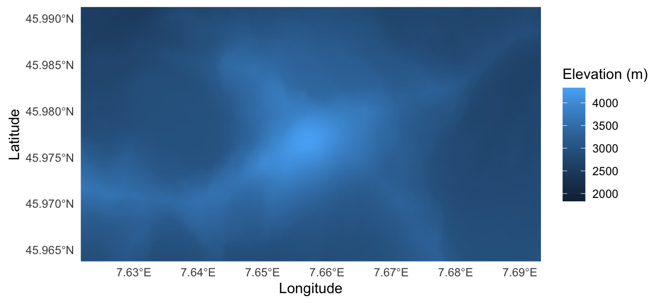
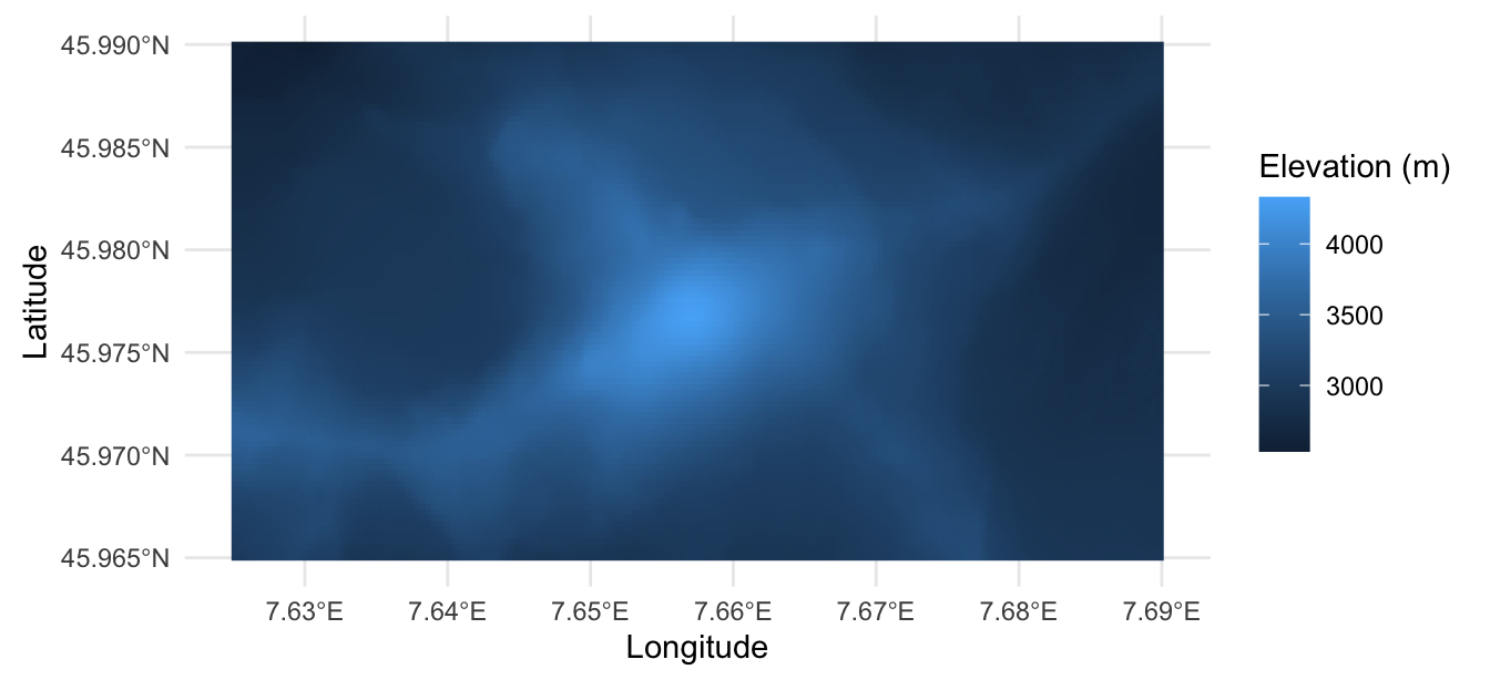
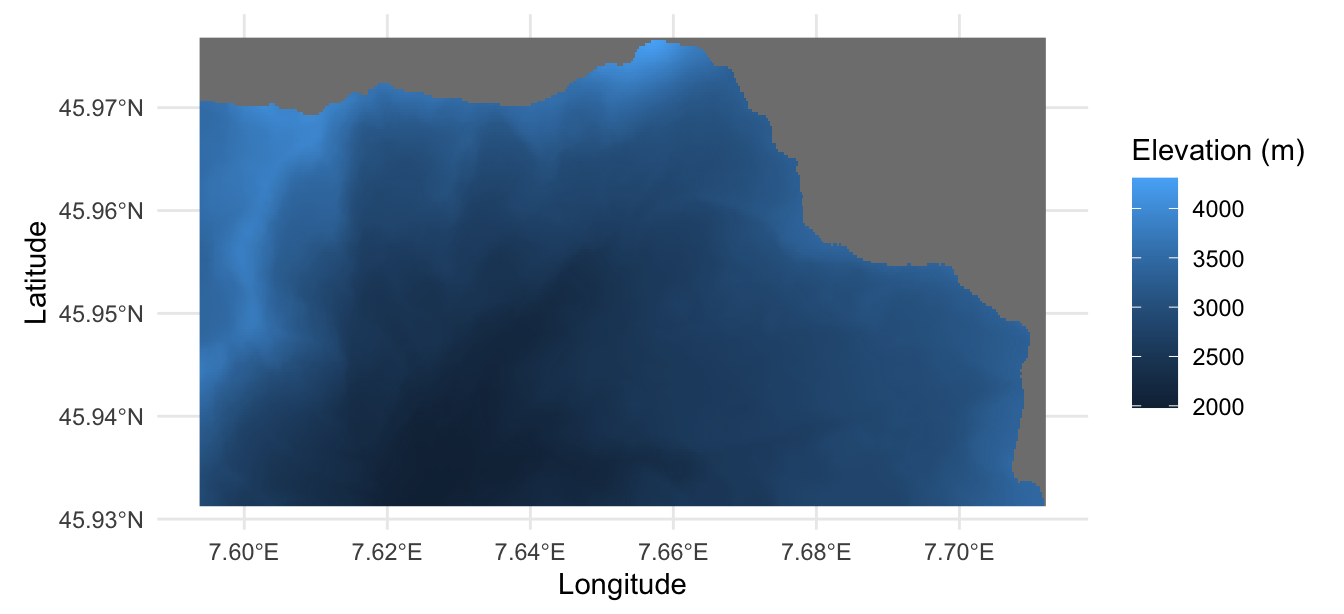
When visualizing geospatial rasters, we sometimes want to focus on a particular geographic region rather than the entire dataset. In this section, we consider three approaches. Zooming changes the area displayed on the map without altering the underlying raster. Cropping retains a rectangular subset of the raster, while masking replaces cell values outside a selected region with missing values (NA), allowing us to isolate areas with irregular boundaries.
To compare zooming and cropping, we select a rectangular region, outlined in red in Figure 17.3, around the Matterhorn summit. We then use the Swiss–Italian border to demonstrate masking.
region <- st_bbox(
  c(xmin = 7.625, xmax = 7.690, ymin = 45.965, ymax = 45.990),
  crs = st_crs(matterhorn_dem)
)
gg_matterhorn <- function(raster) {
  ggplot() +
    geom_stars(data = raster) +
    labs(x = "Longitude", y = "Latitude", fill = "Elevation (m)") +
    theme_minimal()
}
gg_matterhorn(matterhorn_dem) +
  geom_sf(
    data = st_as_sf(st_as_sfc(region)),
    fill = NA,
    color = "red",
    linewidth = 2
  ) +
  coord_sf(crs = st_crs(matterhorn_dem))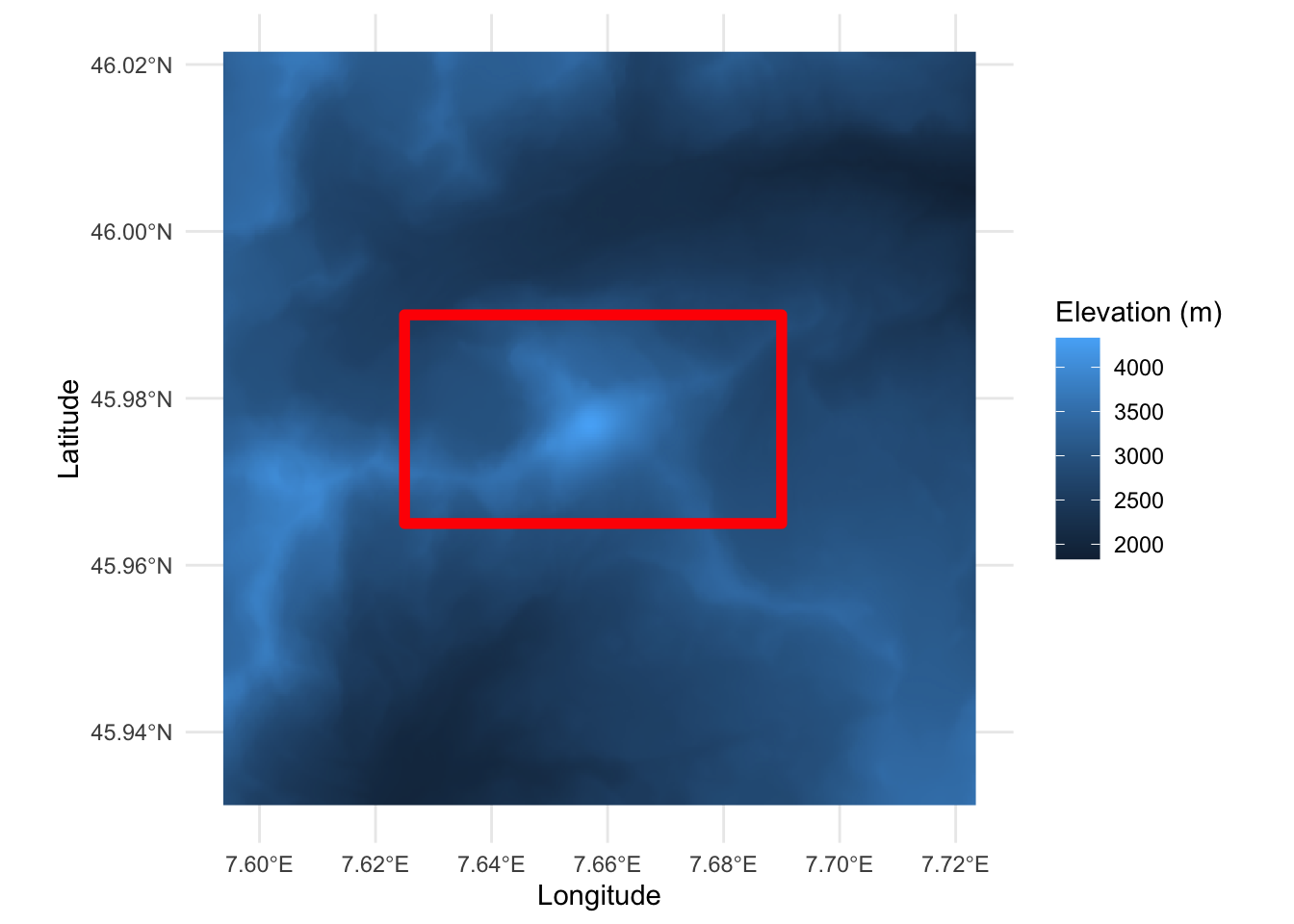
17.5.1 Zooming to a Specific Area
17.5.2 Cropping to a Bounding Box
17.5.3 Masking with a Polygon
The Matterhorn stands on the border between Switzerland and Italy, so we use a polygon of the Swiss national territory to demonstrate masking:3
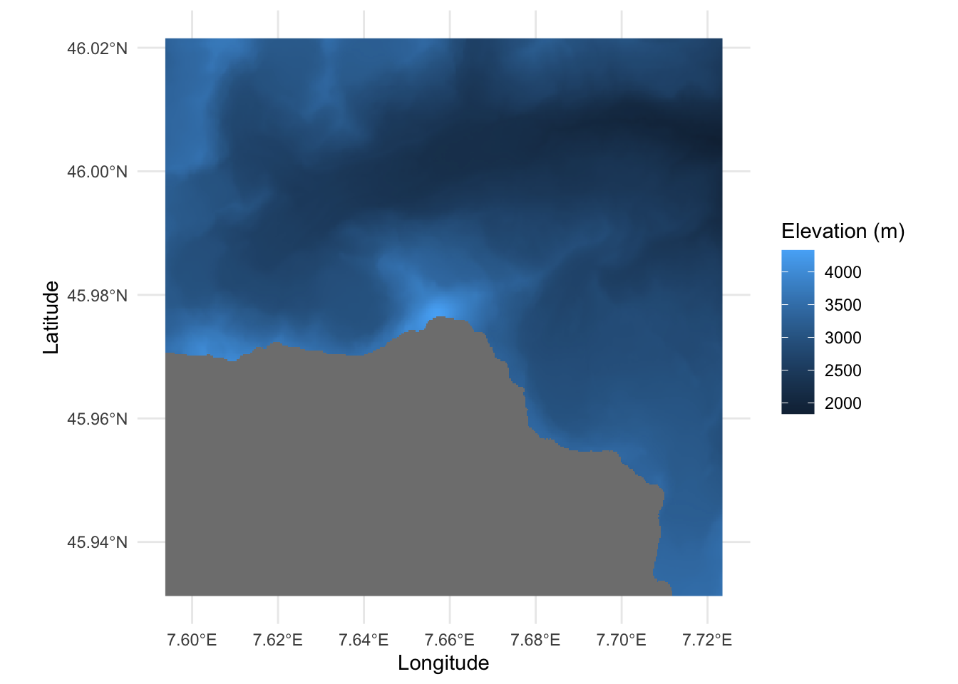
outside_switzerland <- matterhorn_dem |>
  st_bbox() |>
  st_as_sfc() |>
  st_difference(st_geometry(switzerland))
outside_mask <- st_crop(
  matterhorn_dem,
  outside_switzerland,
  crop = FALSE
)
gg_matterhorn(outside_mask) +
  coord_sf(crs = st_crs(outside_mask))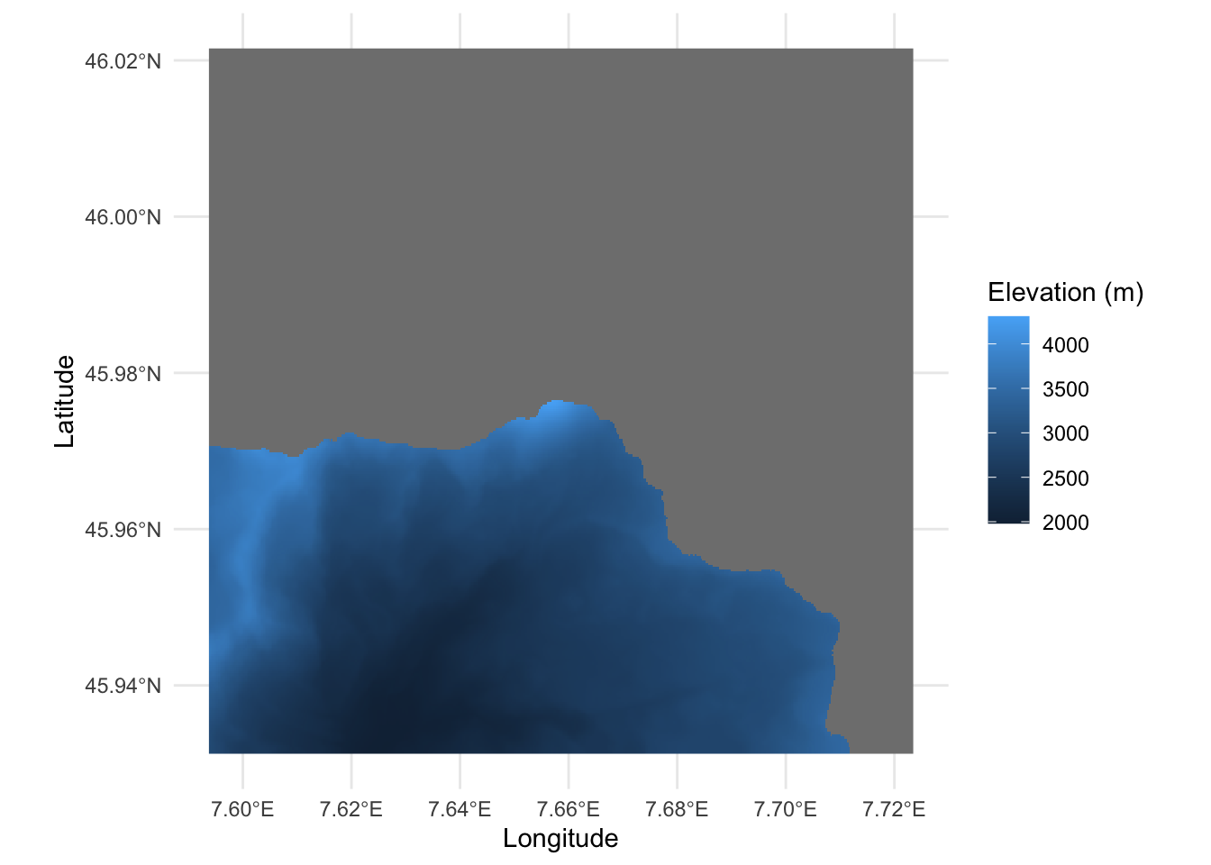
17.6 Missing Data
17.7 Transforming Values and Dimensions
17.8 Changing the Grid: Resolution, Alignment, and Coordinate Reference System
17.9 Choosing a Suitable Palette
17.10 Terrain Visualization
17.11 Conclusion
Produced using Copernicus WorldDEM-30 © DLR e.V. 2010–2014 and © Airbus Defence and Space GmbH 2014–2018, provided under COPERNICUS by the European Union and ESA; all rights reserved. The organisations in charge of the Copernicus programme by law or by delegation do not incur any liability for any use of the Copernicus WorldDEM-30.↩︎
Contains modified Copernicus Sentinel data 2023.↩︎
Source: Federal Office of Topography swisstopo. The polygon is taken from the swissBOUNDARIES3D dataset (release 2026-01), with elevations removed and coordinates converted to longitude and latitude.↩︎